Optimization of RANS Coefficients for Steady and Decelerating Turbulent Jets

Youngik Song; Vlad Aparece-Scutariu; Dong-hyuk Shin

doi:10.6108/JPNE.2025.5.1.001

Preview

Research Article

Journal of Propulsion and Energy. 31 May 2025. 1-21
https://doi.org/10.6108/JPNE.2025.5.1.001

Optimization of RANS Coefficients for Steady and Decelerating Turbulent Jets

Youngik Song^a

Vlad Aparece-Scutariu^b

Dong-hyuk Shin^a^*

^aDepartment of Aerospace Engineering, KAIST, 291 Daehak-ro, Yuseong-gu, Daejeon 34141, Korea

^bRomanian Research and Development Institute for Gas Turbines COMOTI, Bucharest 061126, Romania

^{*Corresponding Author}

ABSTRACT

The RANS model is optimized for steady and decelerating axisymmetric turbulent jets. The $k - ε$ model was found to be the most suitable candidate for optimization, and two optimized coefficient sets were developed as a result. Each set minimizes the sum of root mean square errors, with one set focused on mean velocities and the other on both mean velocities and Reynolds shear stress. The self-similarity of standard and optimized RANS coefficient sets was then investigated. The optimized sets demonstrated improved self-similarity over the standard coefficient set, showing a close match with a $C_{a}$ value of 2.2.

Keywords

Turbulence

Computational fluid dynamics (CFD)

Reynolds-Averaged Navier-Stokes (RANS)

Jet

Decelerating

MAIN

1. Introduction
1.1 Background
2. Methodology
2.1 Analysis
2.2 Tam-Thies $k - ω$ SST model
2.3 Simulation Details
3. Results and Discussion
3.1 Optimal RANS model candidate
3.2 Coefficient optimization for $k - ε$ model
3.2 Self-similarity of optimized $k - ε$ models
4. Conclusion
Appendix

1. Introduction

1.1 Background

The turbulent jet is an important fluid phenomenon for the propulsion of gas turbines. A turbulent jet is often simulated using computational fluid dynamics (CFD) methods to predict the behavior of fluid at fuel injection [1], and cooling of the engine through the injection of air or water into the turbine [2]. Also, jet plumes from engines have been the subject of aero-acoustic analysis for the reduction of noise. A transient jet, where the inlet velocity decelerates from a steady-state turbulent jet, has been widely studied for applications such as fuel injection in diesel engines [3] and volcanic eruptions [4].

Direct numerical simulations (DNS) by Shin et al. [5] and Craske and Van Reeuwijk [6], as well as experiments by Borée et al. [7] and Witze [8], have been conducted on decelerating jets. Models for unsteady jets and plumes have also been developed. Morton et al. [9] proposed a model for steady axisymmetric plumes, assuming self-similarity of mean axial velocity and mean buoyancy force. Additional modeling of unsteady jets has been carried out by Scase et al. [10], Craske and Van Reeuwijk [11], Musculus [3], and Shin et al. [5]. Unsteady turbulent plume problems have also been examined by Wise and Hunt [12], Scase et al. [13,14], Craske and Van Reeuwijk [6,15].

Craske and Van Reeuwijk [11] suggested using governing equations based on mean energy conservation as an alternative to the classical mass-momentum formulation, without relying on self-similarity. However, models by Musculus [3], Craske and Van Reeuwijk [6], Scase et al. [10,13,14] assume self-similarity as the basis of their models, demonstrating this assumption to be useful. Although many models for unsteady turbulent jets and plumes assume self-similarity, Shin et al. [5] showed that a model based on the self-similarity assumption aligns well with simulation data for the normalized velocity moments profile of decelerating jets.

The Reynolds-Averaged Navier-Stokes (RANS) model is widely used to predict the behavior of turbulent flows at a relatively low computational cost. Bardina et al. [16] validated RANS models across various flows and concluded that the $k - ε$ and $k - ω$ SST models perform best for jet flows, although they tend to overpredict the spreading rate of circular jets, a limitation known as the plane and circular jet anomaly. Georgiadis et al. [17] tested various RANS models to verify their predictions for jet flow from a lobed nozzle. Similarly, Koch et al. [18] applied the $k - ε$ model to an axisymmetric jet from a two-stream nozzle and found good agreement, though with an under-prediction of turbulent kinetic energy.

Due to the limitations of the RANS turbulence model, as noted by Spalart [19], specifically that a universal coefficient for arbitrary flows does not exist, research has been focused on optimizing the model by adjusting its coefficient set for various flow types. Ray et al. [20] and Morgans et al. [21] each conducted coefficient calibration of $k - ε$ and $k - ω$ models for jets in crossflow, while Givi and Ramos [22] modified the $k - ε$ model coefficients for a better approximation of jet spreading rates.

To address the plane and circular jet anomaly and improve the predictability of circular jets, Pope [23] suggested adding a vortex stretching term to the $k - ε$ model to enhance the spreading rate prediction for round jets. Thies and Tam [24] modified the model’s coefficients for compressible flows, creating the Tam-Thies model and subsequently the Tam and Ganesan model [25] for heated jets. The Tam-Thies model showed better alignment with experimental data than the standard $k - ε$ and $k - ω$ SST models, though it produced significantly lower levels of turbulence kinetic energy [26]. Recently, Li et al. [27] further adapted the Tam-Thies model into an SST formulation suited for simulating round jets in near-wall regions, with the specific aim of improving impinging jet predictions.

This paper aims to improve the RANS model for jet flows that decelerate to zero. Four different turbulence models are benchmarked using standard coefficient sets, and the model with the lowest sum of root mean square errors is selected through an iterative process. Two optimization modes are conducted to create new coefficient sets: one focused on reducing mean velocity errors and other on reducing errors in both mean velocities and Reynolds shear stress. The self-similar properties of the optimized models are then verified.

2. Methodology

2.1 Analysis

The Navier-Stokes equations in cylindrical coordinates are formulated as follows [28]:

(1)

\frac{\partial \bar{u_{x}}}{\partial x} + \frac{1}{r} \frac{\partial (r \bar{u_{r}})}{\partial r} = 0

(2)

\frac{\partial \bar{u_{x}}}{\partial t} + \bar{u_{x}} \frac{\partial \bar{u_{x}}}{\partial x} + \bar{u_{r}} \frac{\partial \bar{u_{x}}}{\partial r} = ν (\frac{1}{r} \frac{\partial \bar{u_{x}}}{\partial r} + \frac{\partial^{2} \bar{u_{x}}}{\partial r^{2}} + \frac{\partial^{2} \bar{u_{x}}}{\partial x^{2}}) - \frac{\partial \bar{(u_{x}^{'} u_{x}^{'}})}{\partial x} - \frac{1}{r} \frac{\partial (r \bar{u_{x}^{'} u_{r}^{'}})}{\partial r} - \frac{1}{ρ} \frac{\partial \bar{p}}{\partial x}

(3)

\frac{\partial \bar{u_{r}}}{\partial t} + \bar{u_{x}} \frac{\partial \bar{u_{r}}}{\partial x} + \bar{u_{r}} \frac{\partial \bar{u_{r}}}{\partial r} = ν (- \frac{\bar{u_{r}}}{r^{2}} + \frac{1}{r} \frac{\partial \bar{u_{r}}}{\partial r} + \frac{\partial^{2} \bar{u_{r}}}{\partial r^{2}} + \frac{\partial^{2} \bar{u_{r}}}{\partial x^{2}}) - \frac{\partial (\bar{u_{x}^{'} u_{r}^{'}})}{\partial x} - \frac{1}{r} \frac{\partial (r \bar{u_{r}^{'} u_{r}^{'}})}{\partial r} - \frac{1}{ρ} \frac{\partial \bar{p}}{\partial r}

From these equations, flow properties can be expressed using shape functions based on the self-similarity assumption [5]:

(4)

\bar{u_{x}} = \bar{u_{c}} f (η), \bar{u_{r}} = \bar{u_{c}} g (η), \bar{u_{x}^{'} u_{r}^{'}} = {\bar{u_{c}}}^{2} h (η), \bar{u_{x}^{'} u_{x}^{'}} + \frac{\bar{p} - p_{0}}{ρ} = {\bar{u_{c}}}^{2} k (η)

The central axial velocity $\bar{u_{c}}$ can be expressed in terms of axial distance, time, a virtual time origin $t_{0}$ , and a constant $C_{a, c e n t e r}$ :

(5)

\bar{u_{c}} = \frac{x}{C_{a, center} (t - t_{0})}

The self-similarity constant related to the temporal evolution of the axial velocity at the centerline is specified as $C_{a, c e n t e r}$ . The following equations are related to $C_{a}$ :

(6)

C_{a, d i f f} = f - η \frac{\partial f}{\partial η} + \frac{g}{f} \frac{\partial f}{\partial η} + \frac{1}{η f} \frac{\partial (η h)}{\partial η} + \frac{2 k}{f} - \frac{η}{f} \frac{\partial y}{\partial η}

(7)

C_{a, i n t} = \frac{4 \int_{0}^{\infty} f^{2} η d η + 4 \int_{0}^{\infty} k η d η}{\int_{0}^{\infty} f η d η}

(8)

h = \frac{C_{a, shear}}{η} \int_{0}^{η} η^{'} f d η^{'} + \frac{4}{η} \int_{0}^{η} η^{'} f^{2} d η^{'} + \frac{3 f}{η} \int_{0}^{η} η^{'} f d η^{'} + η k - \frac{4}{η} \int_{0}^{η} η^{'} k d η^{'}

(9)

\frac{\partial h (0)}{\partial η} = \frac{(C_{a, g r a d} - 1)}{2} + k (0)

We denote the values of $C_{a}$ obtained from different equations with specific subscripts. Equation 6 reorganizes the momentum equation under a high Reynolds number assumption to obtain $C_{a, d i f f}$ , while equation 7 integrates to yield $C_{a, i n t}$ . Equation 8 is derived by applying equation 5 to the momentum equation, using $C_{a, s h e a r}$ to express shear stress through the mean velocity profile, and equation 9 derives $C_{a, g r a d}$ by calculating the gradient along the center axis.

2.2 Tam-Thies $k - ω$ SST model

The Tam-Thies $k - ε$ model is a variation of the $k - ε$ model that incorporates an additional vortex stretching term, as suggested by Pope [23], with coefficients adjusted by Thies and Tam [24] to simulate jet spreading rates more accurately. This model has demonstrated superiority over conventional two-equation turbulence models in predicting mean velocity [26]. The governing equations are as follows.

(10)

\frac{\partial (ρ k)}{\partial t} + \frac{\partial (ρ \bar{u_{j}} k)}{\partial x_{j}} = \frac{\partial}{\partial x_{j}} [(μ + \frac{μ_{t}}{σ_{k}}) \frac{\partial k}{\partial x_{j}}] + P_{k} - ρ ϵ

(11)

\frac{\partial (ρ ϵ)}{\partial t} + \frac{\partial (ρ {\bar{u}}_{j} ϵ)}{\partial x_{j}} = \frac{\partial}{\partial x_{j}} [(μ + \frac{μ_{t}}{σ_{ϵ}}) \frac{\partial ϵ}{\partial x_{j}}] + C_{ϵ 1} \frac{ϵ}{k} P_{k} - C_{ϵ 2} ρ \frac{ϵ^{2}}{k} + C_{ϵ 3} ρ X \frac{ϵ^{2}}{k}

where turbulent eddy viscosity is calculated as

(12)

μ_{t} = C_{μ} ρ \frac{k^{2}}{ϵ}

and vortex stretching term X is

(13)

X = \bar{ω_{i j}} \bar{ω_{j k}} \bar{S_{k i}}

with the components defined as:

(14)

\bar{ω_{i j}} = \frac{1}{2} \frac{k}{ϵ} (\frac{\partial {\bar{u}}_{i}}{\partial x_{j}} - \frac{\partial {\bar{u}}_{j}}{\partial x_{i}})

(15)

\bar{S_{i j}} = \frac{1}{2} \frac{k}{ϵ} (\frac{\partial {\bar{u}}_{i}}{\partial x_{j}} + \frac{\partial {\bar{u}}_{j}}{\partial x_{i}})

The standard model parameters of Tam-Thies $k - ε$ model are as follows: $C_{μ}$ =0.087, $C_{ε 1}$ =1.40, $C_{ε 2}$ =2.02, $σ_{k}$ =0.32, $σ_{ε}$ =0.38, and $C_{ε 3}$ =0.82.

The $k - ω$ SST model combines Wilcox’s $k - ω$ model for the near-wall regions with the $k - ε$ model for the far-field region [29]. The SST version of the Tam-Thies model is designed to replace the $k - ε$ model with the Tam-Thies $k - ε$ model in the $k - ω$ SST model framework, retaining the vortex stretching term and allowing simulation of domains with wall-bounded flow. This SST adaptation of the Tam-Thies model was suggested for modeling impinging jet [27]. In this work, it was adopted for the simulation of a turbulent jet from a flat plate without co-flow, since at the simulation using the conventional Tam-Thies $k - ε$ model, the X term has diverged 𝜖 value near the wall and consequentially velocity and pressure. The governing equations are as follows.

(16)

\frac{\partial (ρ k)}{\partial t} + \frac{\partial (ρ {\bar{u}}_{j} k)}{\partial x_{j}} = \frac{\partial}{\partial x_{j}} [(μ + α_{k} μ_{t}) \frac{\partial k}{\partial x_{j}}] + P_{k} - β^{*} ρ ω k

(17)

\frac{\partial (ρ ω)}{\partial t} + \frac{\partial (ρ {\bar{u}}_{j} ω)}{\partial x_{j}} = \frac{\partial}{\partial x_{j}} [(μ + α_{ω} μ_{t}) \frac{\partial ω}{\partial x_{j}}] + \frac{γ}{ν_{t}} P_{k} - β ρ ω^{2} + (1 - F_{1}) (\frac{2 ρ α_{ω 2}}{ω} \frac{\partial k}{\partial x_{j}} \frac{\partial ω}{\partial x_{j}} + C_{X} ρ X ω^{2})

where

(18)

X = \bar{ω_{i j}} \bar{ω_{j k}} \bar{S_{k i}}

with the components defined as:

(19)

\bar{ω_{i j}} = \frac{1}{2} \frac{1}{β^{*} ω} (\frac{\partial {\bar{u}}_{i}}{\partial x_{j}} - \frac{\partial {\bar{u}}_{j}}{\partial x_{i}})

(20)

\bar{S_{i j}} = \frac{1}{2} \frac{1}{β^{*} ω} (\frac{\partial {\bar{u}}_{i}}{\partial x_{j}} + \frac{\partial {\bar{u}}_{j}}{\partial x_{i}})

The general coefficients of the Tam-Thies $k - ε$ model are adapted to derive the coefficients for the SST version of the model as follows:

(21a)

β^{*} = C_{μ}

(21b)

β_{2} = C_{μ} (C_{ε 2} - 1)

(21c)

γ_{2} = C_{ε 1} - 1

(21d)

α_{k 2} = \frac{1}{σ_{k}}

(21e)

α_{ω 2} = \frac{1}{σ_{ε}}

(21f)

C_{X} = C_{μ} C_{ε 3}

The resulting model parameters of Tam-Thies $k - ω$ SST model are as follows: $β^{*}$ =0.087, $β_{2}$ =1.40, $γ_{2}$ =0.4, $α_{k 2}$ =1/0.32, $α_{ω 2}$ =1/0.38, and $C_{X}$ =0.0713. The remaining equations and parameters are identical to those of the $k - ω$ SST model.

2.3 Simulation Details

Numerical simulations were conducted using OpenFOAM 11 with an axisymmetric mesh. A single grid size of 0.02𝜋 radians is in the circumferential direction to reduce the mesh size and replicate a one-hundredth of the cylindrical domain, spanning $x / D$ =0-90 in the axial direction and $r / D$ =0-30 in the radial direction. However, the sharp angle reduces the mesh quality, so the grid study was conducted to resolve this issue.

https://cdn.apub.kr/journalsite/sites/jpne/2025-005-01/N0640050101/images/jpne_2025_51_001_F1.jpg

Fig. 1.

Numerical domain for an axisymmetric turbulent jet.

https://cdn.apub.kr/journalsite/sites/jpne/2025-005-01/N0640050101/images/jpne_2025_51_001_F2.jpg

Fig. 2.

Grid study using $k - ε$ model for steady (a-c) and decelerating (d-f) jet flow.

https://cdn.apub.kr/journalsite/sites/jpne/2025-005-01/N0640050101/images/jpne_2025_51_001_F3.jpg

Fig. 3.

Temporal profiles at 1 𝜏, 11 𝜏, 21 𝜏 for the axial mean velocity of a decelerating jet, where $τ = D / u_{0}$ and time is measured from the onset of velocity deceleration. The simulations used the (a) DNS and (b) $k - ε$ model.

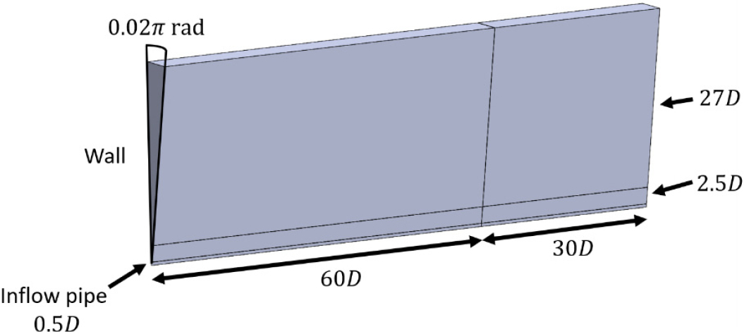
The computational grid consists of three blocks in the radial direction. The first block covers $r / D$ =0-0.5 with cells that have a uniform growth rate, with decreasing mesh size as the radius increases. The second block spans $\frac{r}{D}$ =0.5-3 and also has a uniform growth rate, with increasing mesh size as the radius increases. The final layer, from $r / D$ =3-30 consists of equidistant cells. In the axial direction, the mesh is divided into two blocks: the first block, covering $x / D$ =0-60, consists of cells with a uniform growth rate with increasing mesh size as further from the jet inlet, while the second block, spanning $x / D$ =60-90, is composed of equidistant cell layers. The resulting mesh structure is shown in Fig. 1.

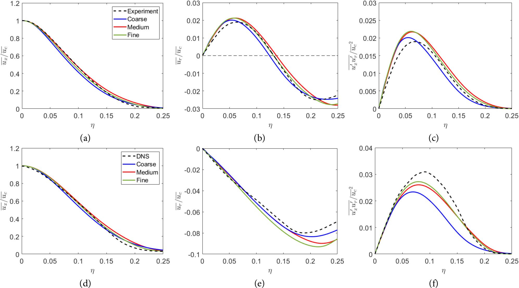
A grid study was conducted using the standard coefficients $k - ε$ turbulence model. The steady-state jet was compared with experimental data from Panchapakesan and Lumley [30], while the decelerating-state jet was validated against DNS data from Shin et al. [5]. The medium mesh size included a layer of 10 cells in the first radial block and 600 cells in the first axial block. Different meshes were studied, including a coarse mesh with 5 cells in the first radial block and 300 cells in the first axial block, as well as a fine mesh with 20 cells in the first radial block and 1200 cells in the first axial block. The medium mesh achieved convergence with the fine mesh, demonstrating its suitability for this research, as shown in Fig. 2.

The radial grid of the selected mesh consists of three blocks. The first block has 10 cells with maximum and minimum cell sizes of $Δ r = 0.080 D$ and $Δ r = 0.032 D$ , respectively. The second block contains 20 cells with maximum and minimum cell sizes of $Δ r = 0.036 D$ and $Δ r = 0.327 D$ , and the final block has 80 cells, each with a cell size of $Δ r = 0.338 D$ . In the axial direction, the mesh consists of two blocks: the first block has 600 cells with maximum and minimum cell sizes of $Δ r = 0.046 D$ and $Δ r = 0.456 D$ , while the second block has 60 cells, each with a cell size of $Δ r = 0.500 D$ .

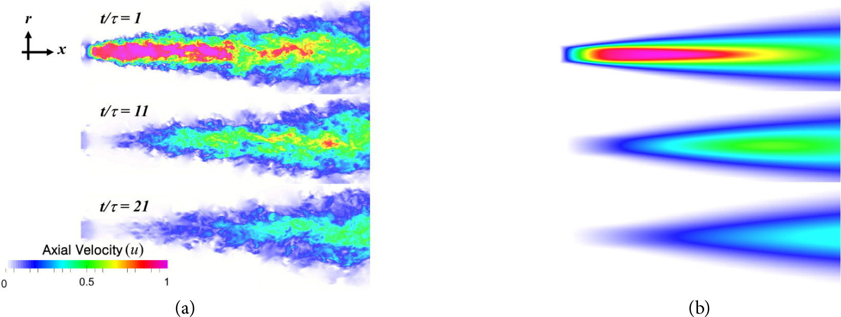
The round jet is exerted with a top-hat velocity profile from a circular inlet at the center of a flat wall into a domain initially filled with stationary fluid, with a Reynolds number of $R e = 7290$ =7290, and a turbulence intensity of 1.7% imposed at the inlet. Far-field and outflow surface boundaries are configured using the outflow boundary condition. The flow was simulated for 620 jet times ( $τ = D / u_{0}$ ) for initialization, after which data for the steady state was sampled over next 380 𝜏, until reaching 1000 𝜏. At 1000 𝜏, the jet inlet velocity started to decrease linearly and reached zero at 1001 𝜏. From this moment, an additional 70 𝜏 of simulation was conducted, and the final 20 𝜏 were sampled for the decelerating state, resulting in the velocity progression shown in Fig. 3 at 1001, 1011, and 1021 seconds (1, 11, and 21 second after deceleration began). Fig. 3b shows RANS data in comparison with DNS data in Fig. 3a from Shin et al. [5].

3. Results and Discussion

3.1 Optimal RANS model candidate

RANS turbulence models were tested for validation on both steady and decelerating jets. The open-source code OpenFOAM was used to solve the Navier-Stokes equations. Among two-equation turbulence models, the $k - ε$ and $k - ω$ SST models were selected, while the Spalart-Allmaras was chosen for a one-equation model. The Tam-Thies $k - ε$ model was also tested, but the result did not converge for a flat plate domain, showing stability only under co-flow conditions. Consequently, the Tam-Thies $k - ω$ SST model was used as an alternative.

The simulation error, compared to experimental steady-state data [30] and DNS results for the decelerating state [5], was quantified using the normalized root mean square error (RMSE), as defined by equation 22 for the scalar Y. The RMSE between the URANS and reference data across the radial range of 𝜂=0-0.25 was computed using first-order numerical integration, and normalized by the amplitude of the reference data.

(22)

E_{Y} = \frac{1}{Y_{r e f, \max} - Y_{r e f, \min}} \sqrt{\frac{1}{0.25} \int_{0}^{0.25} {(Y (η) - Y_{r e f} (η))}^{2} d η}

https://cdn.apub.kr/journalsite/sites/jpne/2025-005-01/N0640050101/images/jpne_2025_51_001_F4.jpg

Fig. 4.

URANS results for steady (a-c) and decelerating (d-f) jet flows.

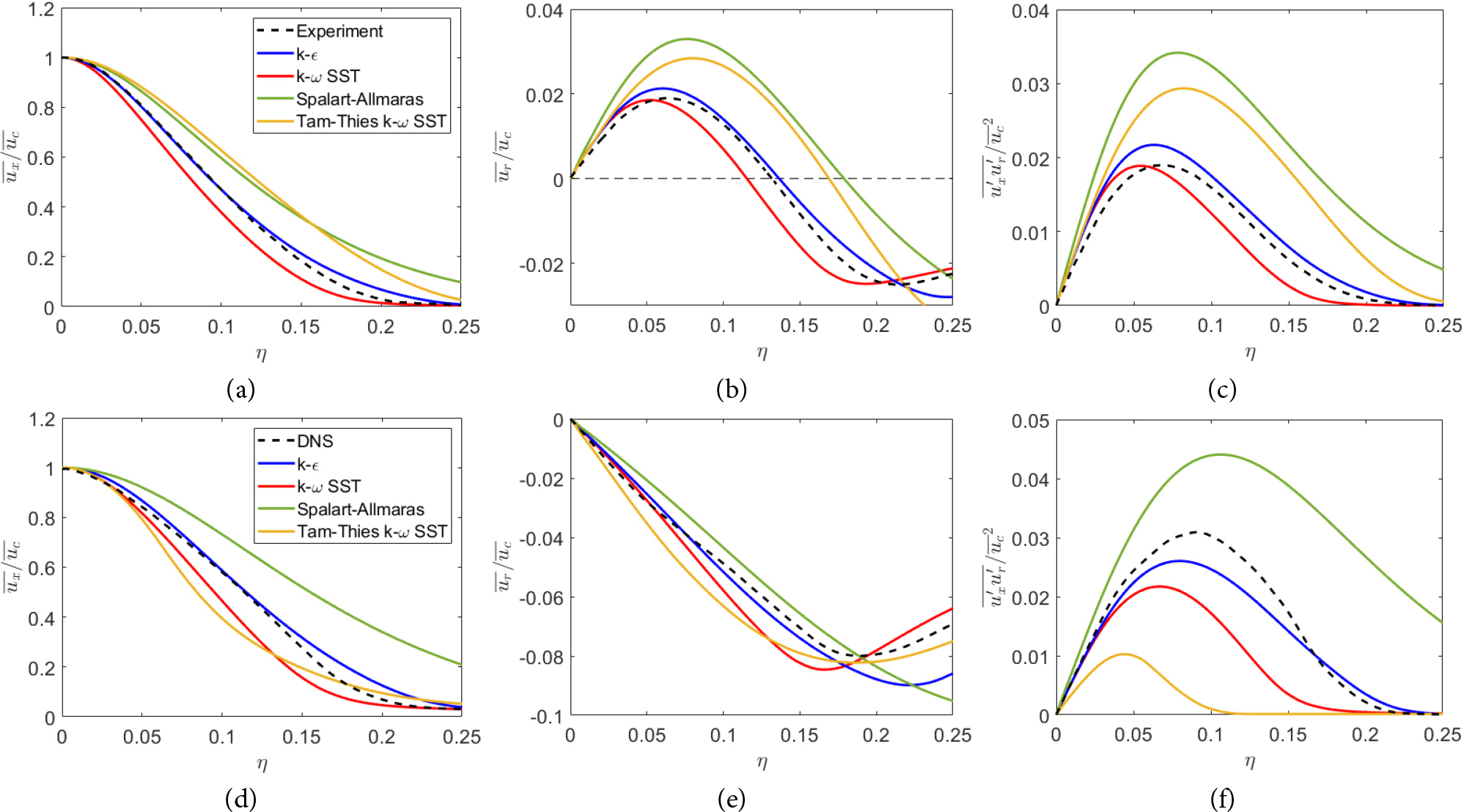
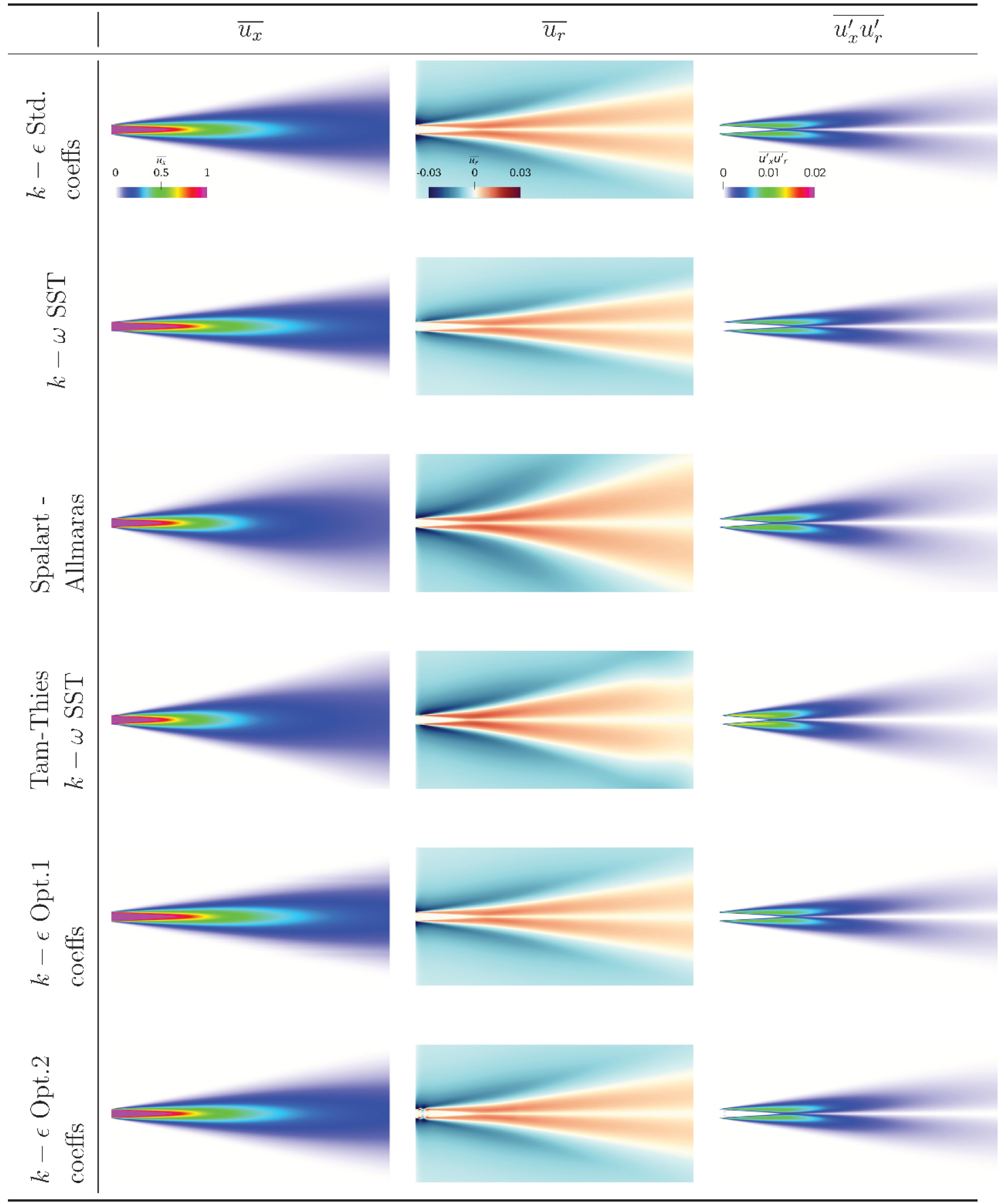
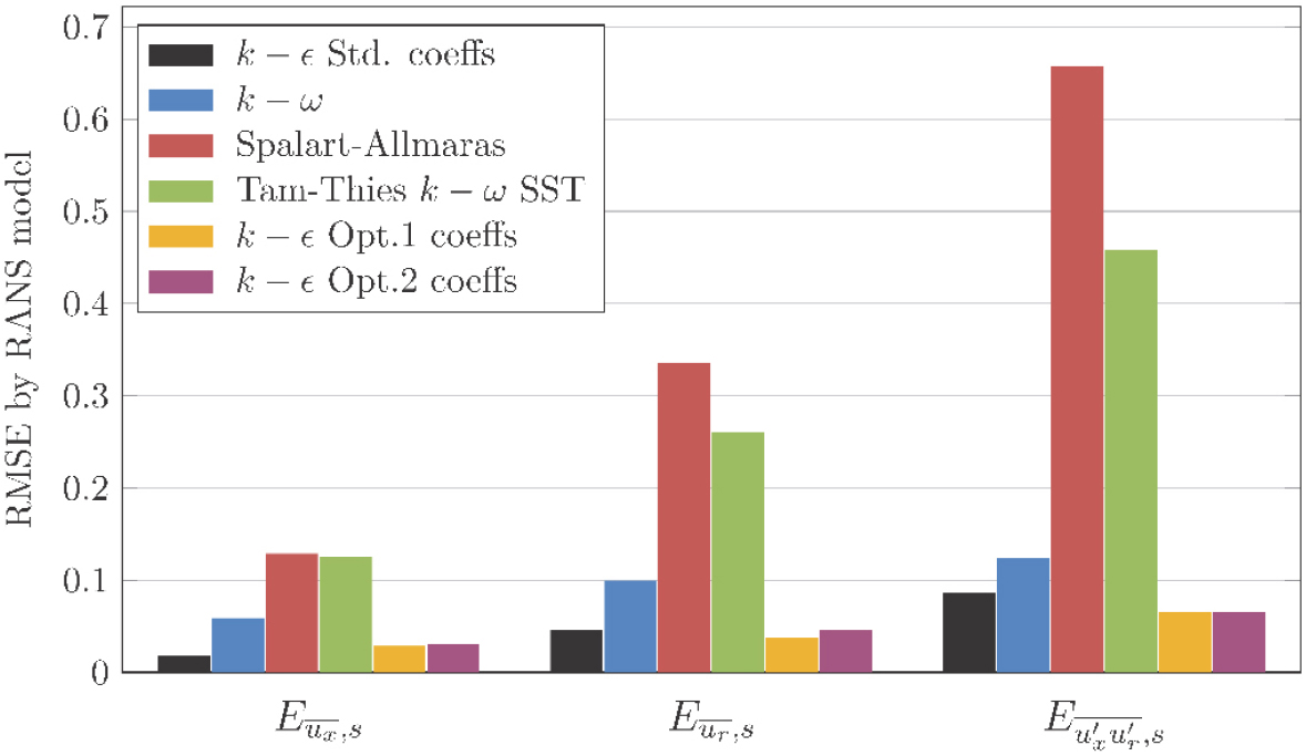
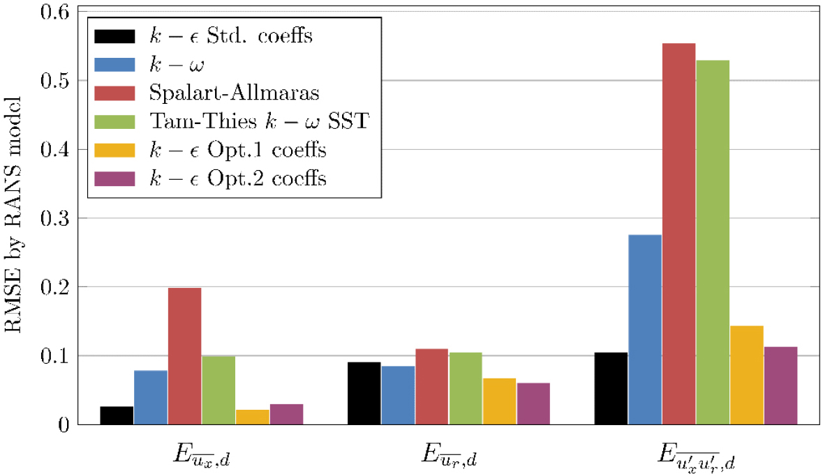
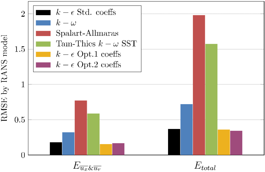
Fig. 4 shows the results of various RANS turbulence models with their default coefficients. Figs. 4a-4c compare the models for a steady axisymmetric jet, while Figs. 4d-4f show comparisons for a decelerating jet. Errors for the axial velocity $\bar{u_{x}}$ , radial velocity $\bar{u_{r}}$ , and Reynolds shear stress $\bar{u'_{x} u'_{r}}$ were calculated for both steady and decelerating states. The resulting errors for each plot and their summations are presented in Table 1. These errors are further compared across steady jet simulations in Fig. 5, decelerating jet simulations in Fig. 6, and the summation of errors in Fig. 7. Here, $E_{\bar{u_{x}} & \bar{u_{r}}}$ denotes the summation of the four mean velocity errors, as defined in equation 23, and $E_{t o t a l}$ represents the total of all six errors, as described in equation 24.

(23)

E_{\bar{u_{x}} & \bar{u_{r}}} = E_{\bar{u_{x}}, s} + E_{\bar{u_{x}}, d} + E_{\bar{u_{r}}, s} + E_{\bar{u_{r}}, d}

(24)

E_{total} = E_{\bar{u_{x}}, s} + E_{\bar{u_{x}}, d} + E_{\bar{u_{r}}, s} + E_{\bar{u_{r}}, d} + E_{\bar{u_{x}^{'} u_{r}^{'}}, s} + E_{\bar{u_{x}^{'} u_{r}^{'}}, d}

The one-equation Spalart-Allmaras model showed inferior results compared to two-equation $k - ε$ and $k - ω$ SST models, as observed by Bardina et al. [16], displaying high error summations in both steady and decelerating jets. The Tam-Thies $k - ω$ SST model performed reasonably better than the Spalart-Allmaras model but worse compared to other two-equation models. Notably, the vortex stretching effect emerged as a drawback, leading to a significant underestimation of the Reynolds shear stress values in the decelerating state. Unmodified, conventional two-equation RANS models demonstrated the best results, with the lowest overall errors. Among these, the $k - ε$ turbulence model showed the lowest errors for both $E_{\bar{u_{x}} & \bar{u_{r}}}$ and $E_{t o t a l}$ , making it the preferred model for coefficient optimization.

Table 1.

Error values for standard and optimized RANS models for steady (subscript s) and decelerating (subscript d) jets, showing errors for mean velocity, Reynolds shear stress, mean velocity error summation, and total error summation.

Models	Steady jet			Decelerating jet			Summations
Models	$E_{\bar{u_{x}}, s}$	$E_{\bar{u_{r}}, s}$	$E_{\bar{u'_{x} u'_{r}}, s}$	$E_{\bar{u_{x}}, d}$	$E_{\bar{u_{r}}, d}$	$E_{\bar{u'_{x} u'_{r}}, d}$	$E_{\bar{u_{x}} & \bar{u_{r}}}$	$E_{t o t a l}$
$k - ε$ Std. coeffs	0.0169	0.0457	0.0859	0.0258	0.0898	0.1037	0.1782	0.3678
$k - ω$ SST	0.0583	0.0988	0.1237	0.0776	0.0840	0.2746	0.3185	0.7168
Spalart-Allmaras	0.1280	0.3349	0.6567	0.1975	0.1092	0.5533	0.7696	1.9796
Tam-Thies $k - ω$ SST	0.1246	0.2591	0.4570	0.0978	0.1043	0.5290	0.5858	1.5718
$k - ε$ Opt.1 coeffs	0.0278	0.0369	0.0647	0.0204	0.0665	0.1429	0.1516	0.3592
$k - ε$ Opt.2 coeffs	0.0295	0.0449	0.0652	0.0652	0.0600	0.1123	0.1639	0.3414

https://cdn.apub.kr/journalsite/sites/jpne/2025-005-01/N0640050101/images/jpne_2025_51_001_F5.jpg

Fig. 5.

Error values compared for standard and optimized RANS models for steady jet.

https://cdn.apub.kr/journalsite/sites/jpne/2025-005-01/N0640050101/images/jpne_2025_51_001_F6.jpg

Fig. 6.

Error values compared for standard and optimized RANS models for decelerating jet.

https://cdn.apub.kr/journalsite/sites/jpne/2025-005-01/N0640050101/images/jpne_2025_51_001_F7.jpg

Fig. 7.

Summation of error values for standard and optimized RANS models for steady and decelerating jets.

3.2 Coefficient optimization for $k - ε$ model

The $k - ε$ model was optimized for both steady and decelerating jets, following an iterative procedure shown in Fig. 8. The optimization begins with an initial coefficient set $c^{0} = [c_{1}^{0}, c_{2}^{0}, c_{3}^{0}, c_{4}^{0}, c_{5}^{0}]$ , corresponding to the standard $k - ε$ model values $[c_{μ}, c_{1}, c_{2}, σ_{k}, σ_{ε}] = [0.090, 1.44, 1.92, 1.0, 1.3]$ .

In each iteration, the error $E_{i}^{n}$ is calculated by changing only one variable $c_{i}^{n}$ from the coefficient set $c^{n}$ . We then search for the value $\tilde{c_{i}^{n}}$ that minimizes the error $\tilde{E_{i}^{n}}$ . The iteration spans the coefficients with specific intervals: 10^-3 for $c_{μ}$ , 10^-2 for $c_{1}$ and $c_{2}$ , and 10^-1 for $σ_{k}$ and $σ_{ε}$ . This process yields five new sets, each with a different modified coefficient, and five corresponding errors.

Among these errors, the smallest error $\tilde{E_{i}^{n}}$ is identified, along with the associated modified coefficient $\tilde{c_{i}^{n}}$ . The coefficient set that produces this smallest error, $[c_{1}^{n}, \dots \tilde{c_{i}^{n}} \dots c_{5}^{n}]$ is designated as the new default coefficient set $c^{n + 1}$ , and the error $\tilde{E_{i}^{n}}$ becomes $E^{n + 1}$ for $c^{n + 1}$ . The iteration of creating new coefficient sets is repeated until $E^{n + 1}$ is equal to $E^{n}$ and the minimum error remains unchanged. At this point, the iteration stops, and the final set becomes the optimized coefficient set for the decelerating jet.

Two different optimized coefficient sets other than the standard coefficient set (Std.) were created, each using a different criterion for calculating the error of the coefficient set. The first optimized coefficient set (Opt.1) was created by minimizing $E_{\bar{u_{x}} & \bar{u_{r}}}$ , and the second optimized coefficient set (Opt.2) was created by minimizing $E_{t o t a l}$ .

The optimization process for Opt.1 was conducted over two iteration steps, as shown in Fig. 9. In iteration 1, the lowest error for each coefficient was as follows: $c_{μ}$ produced an error of 0.1539 at a value of 0.084, $c_{1}$ resulted in 0.1736 at a value of 1.45, $c_{2}$ yielded 0.1516 at a value of 1.90, $σ_{k}$ produced 0.1782 at a value of 1.0, and $σ_{ε}$ produced 0.1770 at a value of 1.2. The modified coefficient set $c^{1} = [0.090, 1.44, 1.90, 1.0, 1.3]$ with an error $E^{1}$ =0.1516 was selected, and in iteration 2, all coefficients showed the same lowest error as $E^{1}$ for the default set $c^{1}$ , concluding the process.

https://cdn.apub.kr/journalsite/sites/jpne/2025-005-01/N0640050101/images/jpne_2025_51_001_F8.jpg

Fig. 8.

Flowchart illustrating the iterative process for optimizing the turbulence model coefficients.

https://cdn.apub.kr/journalsite/sites/jpne/2025-005-01/N0640050101/images/jpne_2025_51_001_F9.jpg

Fig. 9.

$E_{\bar{u_{x}} & \bar{u_{r}}}$ for the $k - ε$ model during the iterative optimization procedure. Each row represents one iteration step, with the red circle highlighting the point of lowest error for that step.

https://cdn.apub.kr/journalsite/sites/jpne/2025-005-01/N0640050101/images/jpne_2025_51_001_F10.jpg

Fig. 10.

$E_{t o t a l}$ for the $k - ε$ model during the iterative optimization procedure. Each row represents one iteration step, with the red circle highlighting the point of lowest error for that step.

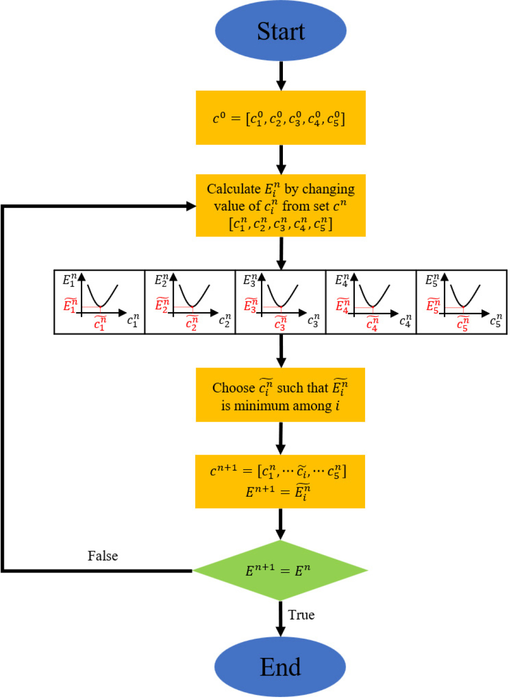
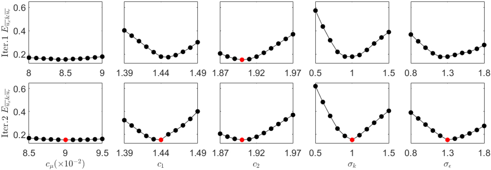
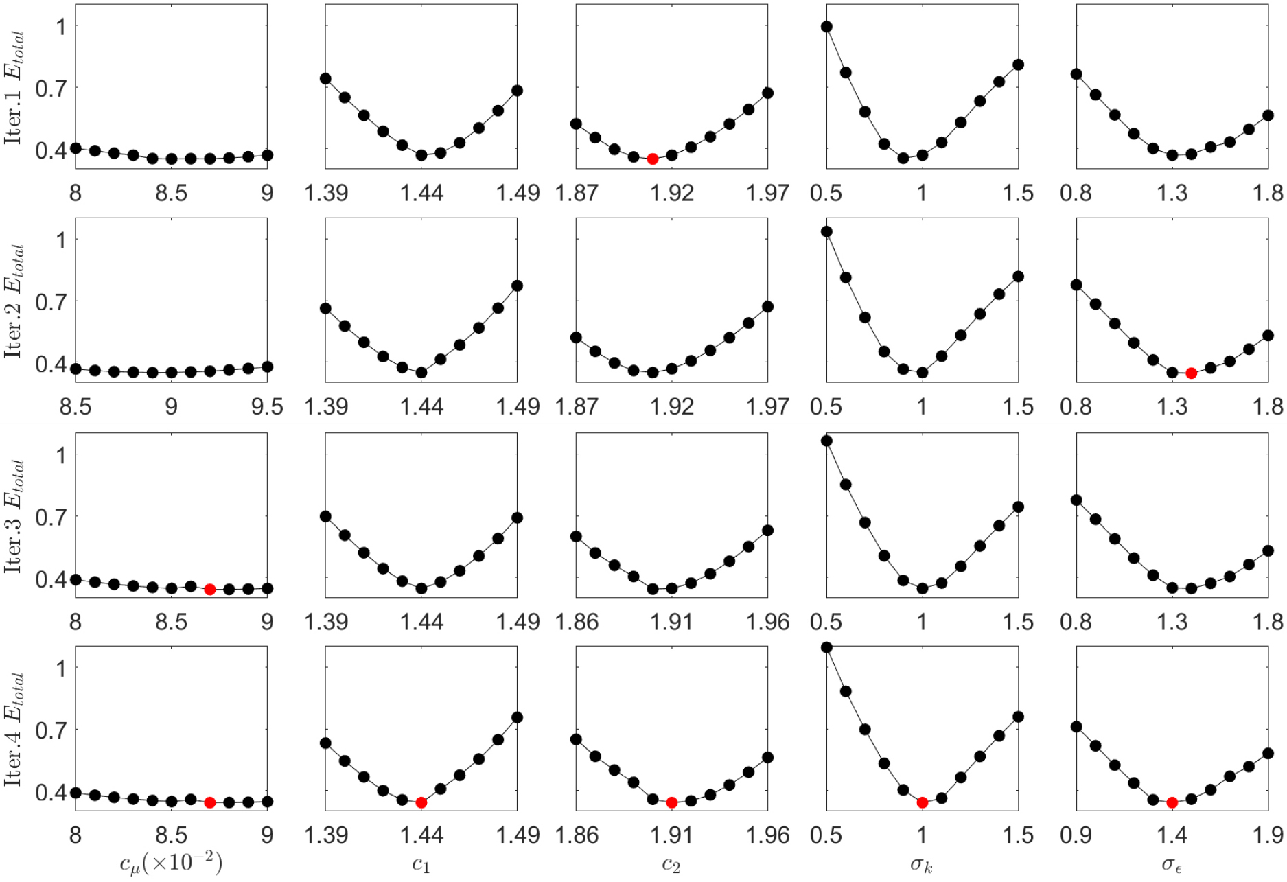
Table 2.

Optimized parameters of the $k - ε$ model for Opt.1 and Opt.2 coefficient sets, alongside the standard coefficient set.

Coefficient	$c_{μ}$	$c_{1}$	$c_{2}$	$σ_{k}$	$σ_{ε}$
$k - ε$ Std. coeffs	0.090	1.44	1.92	1.0	1.3
$k - ε$ Opt.1 coeffs	0.090	1.44	1.90	1.0	1.3
$k - ε$ Opt.2 coeffs	0.087	1.44	1.91	1.0	1.4

The optimization process for Opt.2 was conducted over four iterations steps, as shown in Fig. 10. In iteration 1, the lowest errors for each coefficient were as follows: $c_{μ}$ yielded an error of 0.3497 at a value of 0.085, $c_{1}$ resulted in 0.3678 at a value of 1.44, $c_{2}$ produced 0.3496 at a value of 1.91, $σ_{k}$ resulted in 0.3531 at a value of 0.9, and $σ_{ε}$ yielded 0.3678 at a value of 1.3. The resulting coefficient set $c^{1} = [0.090, 1.44, 1.91, 1.0, 1.3]$ with an error $E^{1}$ =0.3496 was chosen.

In iteration 2 for Opt.2, the lowest errors were as follows: $c_{μ}$ resulted in an error of 0.3492 at a value of 0.089, $c_{1}$ produced 0.3496 at a value of 1.44, $c_{2}$ resulted in 0.3496 at a value of 1.91, $σ_{k}$ produced 0.3496 at a value of 1.0, and $σ_{ε}$ resulted in 0.3464 at a value of 1.4. This modified coefficient set $c^{2} = [0.090, 1.44, 1.91, 1.0, 1.4]$ with an error $E^{2}$ =0.3464 was adopted.

In iteration 3, the lowest errors yielded by each coefficient were as follows: $c_{μ}$ produced an error of 0.3414 at a value of 0.087, $c_{1}$ yielded 0.3464 at a value of 1.44, $c_{2}$ yielded 0.3435 at a value of 1.90, $σ_{k}$ produced 0.3464 at a value of 1.0, and $σ_{ε}$ produced 0.3464 at a value of 1.4. The modified coefficient set $c^{3} = [0.087, 1.44, 1.91, 1.0, 1.4]$ with an error $E^{3}$ =0.3435 was selected. In iteration 4, all coefficients showed the same lowest error as $E^{3}$ with the default coefficient set $c^{3}$ , ending the process.

The resulting optimized coefficient sets, Opt.1 and Opt.2, are shown in Table 2. In Opt.1, only $c_{2}$ differs from the original coefficient set $c^{0}$ . This modification effectively reduced the mean velocity error sum from 0.1782 to 0.1516, narrowing the gap between the model predictions and reference values, except for a slight increase in axial mean velocity error in the steady state.

Although Opt.1 was not specifically optimized to reduce Reynolds shear stress error, it still achieved an overall reduction in total error, decreasing from 0.3678 to 0.3592, particularly improving the steady-state Reynolds shear stress error.

https://cdn.apub.kr/journalsite/sites/jpne/2025-005-01/N0640050101/images/jpne_2025_51_001_F11.jpg

Fig. 11.

Radial profiles for the steady (a-c) and decelerating (d-f) jet flows, comparing optimized and standard $k - ε$ model coefficient sets against experimental data and DNS results.

In Opt.2, the coefficients $c_{2}$ , $σ_{ε}$ , and $c_{μ}$ were modified. As a result, Opt.2 achieved a notable reduction in the total error summation, including both mean velocity and Reynolds shear stress errors, from 0.3678 and 0.3414. Opt.2 showed improved accuracy in radial mean velocity errors and Reynolds shear stress error for the steady state. This improvement in radial mean velocity errors also led to a decrease in the mean velocity error summation, from 0.1782 to 0.1639.

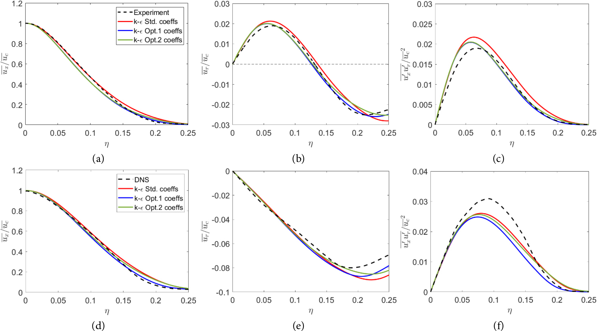
Radial profiles of mean velocities and Reynolds shear stress for the $k - ε$ model, using standard coefficients as well as the optimized sets Opt.1 and Opt.2, are shown in Fig. 11. These profiles are compared with experimental data [30] for the steady state and DNS data [5] for the decelerating state. In the axial mean velocity profiles (Figs. 11a and 11d), the lines representing different coefficient sets are nearly indistinguishable, as the axial mean velocity error was the smallest across all sets.

For the radial mean velocity in (Figs. 11b and 11e), a major discrepancy is observed in the far-field between 𝜂=0.15-0.25. Opt.1 has a higher inflection point but largely maintains the shape of the profile with the standard coefficients, reducing errors in both steady and decelerating state. Meanwhile, Opt.2 shows an inflection point at a similar height but positioned farther from the centerline. This shift in the inflection point improves alignment with DNS data in the decelerating state up to the inflection point, achieving a greater improvement than Opt.1. However, this adjustment has less impact in the steady state, where Opt.1 achieves a larger error reduction.

For Reynolds shear stress (Fig. 11c and 11f), Opt.1 produces a lower peak closer to the centerline for both state, which reduces the error in the steady state but introduces a disadvantage in the decelerating state. Opt.2, with a similar shift but slightly stronger in the steady state, achieves a comparable improvement to Opt.1 in the steady state while exhibiting a smaller increase in error for the decelerating state.

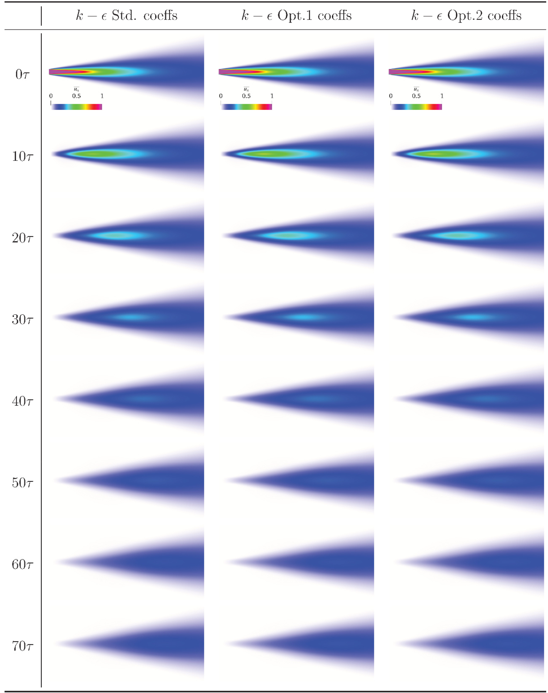
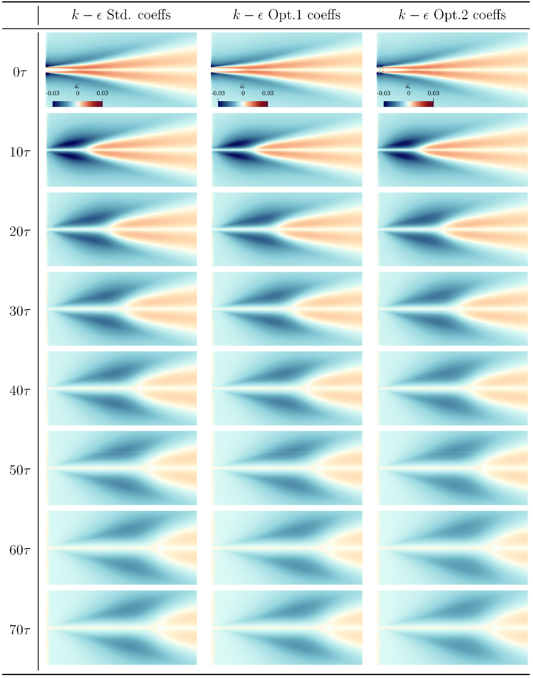
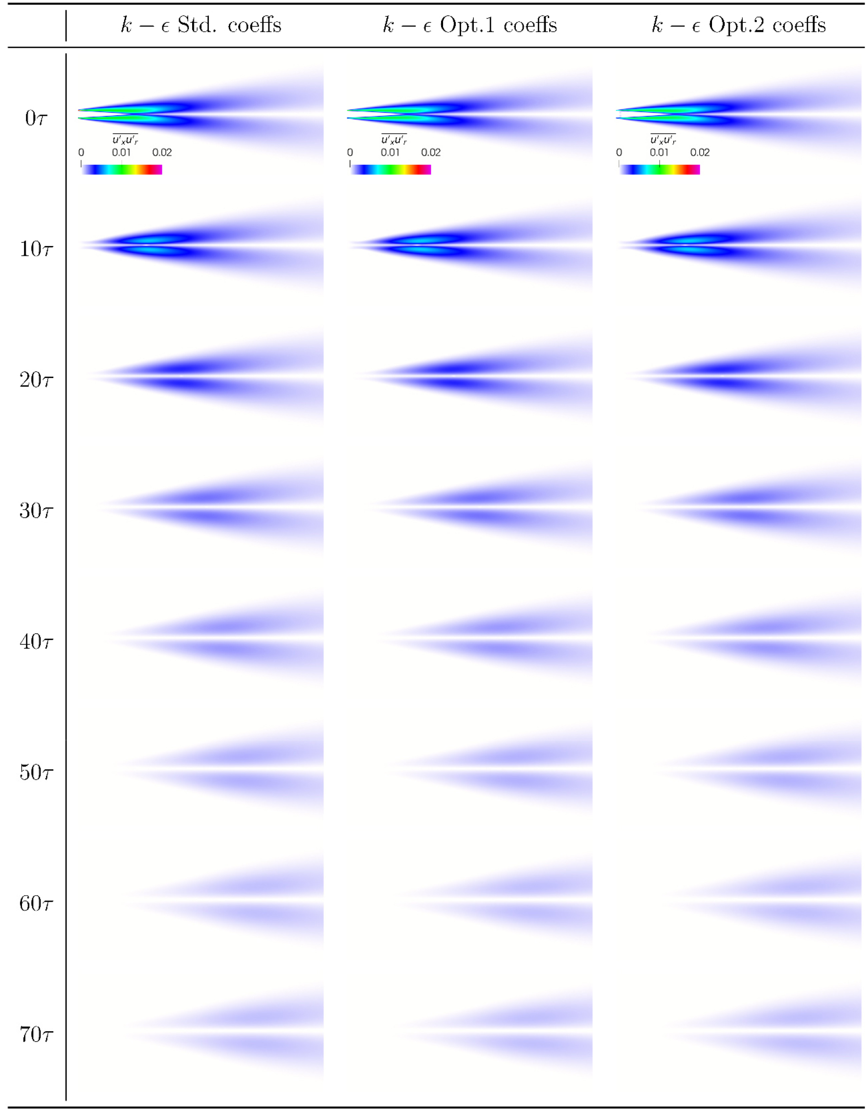
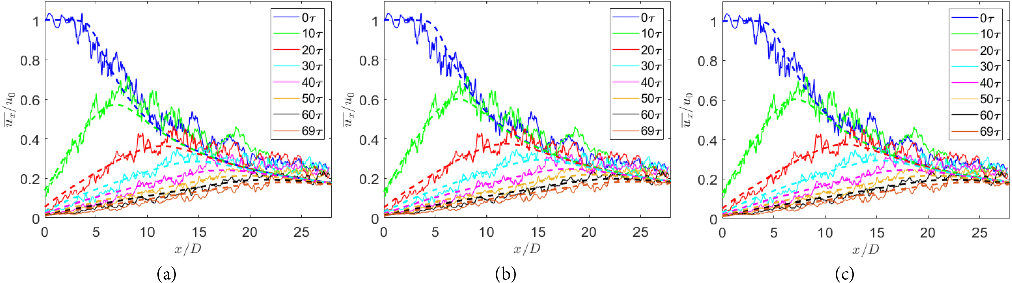
Temporal evolution of the centerline axial mean velocity after the start of deceleration is presented in Fig. 12, with a comparison to DNS data from [5]. The standard coefficient set (Fig. 12a) underpredicts the DNS result. While both optimized coefficients sets, Opt.1 (Fig. 12b) and Opt.2 (Fig. 12c), still fall below the reference DNS data, a slight improvement is evident in both cases.

https://cdn.apub.kr/journalsite/sites/jpne/2025-005-01/N0640050101/images/jpne_2025_51_001_F12.jpg

Fig. 12.

Temporal evolution of centerline axial mean velocity over time for the $k - ε$ model using (a) standard, (b) Opt.1, and (c) Opt.2 coefficient set. The data from RANS is represented with dashed lines, while the DNS results are shown in solid lines.

3.2 Self-similarity of optimized $k - ε$ models

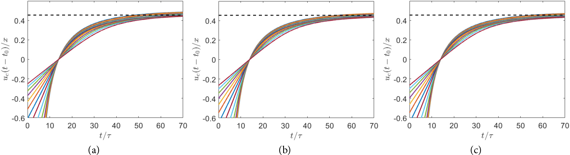
A self-similarity analysis was conducted for both standard and optimized $k - ε$ models. Equation 5 was used to determine the constant $C_{a, c e n t e r}$ , as shown in Fig. 13. Using $t_{0} = 14 / τ$ , consistent with the DNS data from [5] where $τ = D / u_{0}$ , the plot of $1 / C_{a, c e n t e r} = u_{c} (t - t_{0}) / x$ at various axial distances $x / D$ =5-18 (Fig. 13) is shown converging asymptotically near the reference line $1 / C_{a, c e n t e r} \approx 0.455$ , yielding $C_{a, c e n t e r}$ =2.2.

In Figs. 13b and 13c, Opt.1 and Opt.2 asymptotically converged above the reference line, with $C_{a, c e n t e r}$ values of 2.2230 and 2.2454, respectively. In contrast, the standard coefficient set (Fig. 13a) converges slightly below the $C_{a, c e n t e r}$ =2.2 line, resulting in a value of $C_{a, c e n t e r}$ =2.1855. Overall, the $C_{a, c e n t e r}$ values from all three coefficient sets, Std., Opt.1, and Opt.2, closely align with the DNS result.

In addition to $C_{a, c e n t e r}$ , $C_{a}$ was calculated from the DNS and RANS results using three other approaches: $C_{a, g r a d}$ , $C_{a, d i f f}$ , and $C_{a, i n t}$ . $C_{a, d i f f}$ was calculated twice, once including the k term and once neglecting it. For $C_{a, i n t}$ , data integration was performed up to 𝜂=0.5, as this range was determined to be sufficient, with changes in 𝜂 by 0.1 resulting in an impact of less than 1% on the results. Centerline values were used for calculating the other coefficients. The results are summarized in Table 3.

https://cdn.apub.kr/journalsite/sites/jpne/2025-005-01/N0640050101/images/jpne_2025_51_001_F13.jpg

Fig. 13.

Asymptotic convergence of $u_{c} (t - t_{0}) / x$ for the $k - ε$ model using (a) standard, (b) Opt.1, and (c) Opt.2 coefficient sets at $t_{0} = 14 τ$ , shown with the dashed reference line $y$ =1/2.2.

The values for $C_{a, g r a d}$ were 2.1498 for the standard coefficients, 2.1737 for Opt.1, and 2.1953 from Opt.2, showing a lower result with a consistent trend compared to the results for $C_{a, c e n t e r}$ , but higher than the DNS value of 2.0394. For $C_{a, d i f f}$ , the values were slightly higher, with 2.3866 for the standard coefficients, 2.4057 for Opt.1, and 2.4355 for Opt.2, clustering near 2.4. When calculated without the k term, $C_{a, d i f f}$ showed a trend similar to that of $C_{a, c e n t e r}$ and $C_{a, g r a d}$ , with values of 2.1438 for the standard coefficients, 2.1677 for Opt.1, and 2.1892 for Opt.2, though still higher than the DNS data of 2.0676. Conversely, $C_{a, i n t}$ showed the lowest values for DNS data at 1.8193 but yielded the highest values for RANS results, with 2.7649 for the standard coefficient set, 2.8136 for Opt.1, and 2.7782 for Opt.2.

Table 3.

Values of $C_{a}$ calculated using different equations for $k - ε$ models with three different coefficient sets at the centerline, together with result using the DNS data.

Used coeffs.	DNS	$k - ε$ Std. coeffs	$k - ε$ Opt.1 coeffs	$k - ε$ Opt.2 coeffs
$C_{a, c e n t e r}$	2.2	2.1855	2.2230	2.2454
$C_{a, g r a d}$	2.0394	2.1498	2.1737	2.1953
$C_{a, i n t}$	1.8193	2.7649	2.8136	2.7782
$C_{a, d i f f}$	2.0857	2.3866	2.4057	2.4355
$C_{a, d i f f}$ , neglect k	2.0676	2.1438	2.1677	2.1892

4. Conclusion

Four different turbulence models, $k - ε$ , $k - ω$ SST, Spalart-Allmaras, and Tam-Thies $k - ω$ SST were compared against experimental data [30] and DNS data [5] for both steady and decelerating jets. Among these models, the $k - ε$ model was identified as the most suitable candidate and was selected for optimization.

The optimization aimed to minimize the sum of root mean square errors across both steady and decelerating states. Two optimized coefficient sets were developed: Opt.1, which minimizes the sum of four mean velocity errors, and Opt.2, which minimizes the sum of six errors (four mean velocity errors and two Reynolds shear stress errors). The resulting coefficients were $c_{μ}$ =0.090, $c_{1}$ =1.44, $c_{2}$ =1.90, $σ_{k}$ =1.0, and $σ_{ε}$ =1.3 for Opt.1, and $c_{μ}$ =0.087, $c_{1}$ =1.44, $c_{2}$ =1.91, $σ_{k}$ =1.0, and $σ_{ε}$ =1.4 for Opt.2. Both optimized sets successfully minimized their respective target error sums and partially reduced the error for each other’s objectives.

The iteration method used a Gauss-Southwell type coordinate descent method, utilizing an incomplete 1D search to limit the number of coefficient decimal places. However, this led to an inevitable loss of accuracy and increased simulation iterations. Also, since the optimization method is fundamentally an algorithm that searches for local extrema, there is potential for further improvement in identifying global extrema and evaluating the completeness of the optimization. An improved multi-dimensional optimization method such as an artificial neural network (ANN) or response surface model (RSM) can be used for optimization [31], and data-driven methods such as ensemble Kalman filter (EnKF) [27,32] or Bayesian calibration [20] have been used for better accuracy. These enhancements should be explored for future work to advance optimization performance, and apply them to other RANS models to assess their optimization effectiveness.

Self-similarity characteristics of the standard and optimized RANS coefficient sets were then analyzed. The metrics $C_{a, g r a d}$ , $C_{a, c e n t e r}$ , and $C_{a, d i f f}$ , excluding the k term, displayed similar trend, with results from Opt.1 and Opt.2 aligning well with the DNS value of $C_{a}$ =2.2.

Overall, the optimized $k - ε$ model coefficient sets demonstrated improved mean velocity and Reynolds shear stress profiles and aligned well with self-similarity characteristics observed in the DNS data of the decelerating jet.

Acknowledgements

This research was supported (No. N10240104) by Korea Advanced Institute of Science and Technology (KAIST). The authors are grateful for the computational support from the Korea Institute of Science and Technology Information (KISTI) for the Nurion cluster (KSC-2024-CRE-0011). This work was supported by the Romanian Ministry of Research, Innovation and Digitalisation, through the “Nucleu” Programme, part of the National Plan for Research, Development and Innovation, 2022-2027, grant no. PN23.12.02.01.

Appendix

https://cdn.apub.kr/journalsite/sites/jpne/2025-005-01/N0640050101/images/jpne_2025_51_001_FA1.jpg

Appendix Fig. 1.

Steady state profiles of mean velocities and Reynolds shear stress.

https://cdn.apub.kr/journalsite/sites/jpne/2025-005-01/N0640050101/images/jpne_2025_51_001_FA2.jpg

Appendix Fig. 2.

Axial velocity profiles visualized over time after the start of deceleration.

https://cdn.apub.kr/journalsite/sites/jpne/2025-005-01/N0640050101/images/jpne_2025_51_001_FA3.jpg

Appendix Fig. 3.

Radial velocity profiles visualized over time after the start of deceleration.

https://cdn.apub.kr/journalsite/sites/jpne/2025-005-01/N0640050101/images/jpne_2025_51_001_FA4.jpg

Appendix Fig. 4.

Reynolds shear stress profiles visualized over time after the start of deceleration.

References

Li, Y., Kirkpatrick, A., Mitchell, C. and Willson, B., "Characteristic and Computational Fluid Dynamics Modeling of High-Pressure Gas Jet Injection," Journal of Engineering for Gas Turbines and Power, Vol. 126, No. 1, pp. 192-197, 2004.

10.1115/1.1635398

Wang, T. and Dhanasekaran, T.S., "Calibration of a Computational Model to Predict Mist/Steam Impinging Jets Cooling With an Application to Gas Turbine Blades," Journal of Heat Transfer, Vol. 132, No. 122201, 2010.

10.1115/1.4002394

Musculus, M.P.B., "Entrainment Waves in Decelerating Transient Turbulent Jets," Journal of Fluid Mechanics, vol. 638, pp. 117-140, 2009.

10.1017/S0022112009990826

Scase, M.M., "Evolution of Volcanic Eruption Columns," Journal of Geophysical Research, Vol. 114, No. F4, p. 2009JF001300, 2009.

10.1029/2009JF001300

Shin, D.-H., Aspden, A.J. and Richardson, E.S., "Self-similar Properties of Decelerating Turbulent Jets," Journal of Fluid Mechanics, Vol. 833, p. R1, 2017.

10.1017/jfm.2017.600

Craske, J. and Van Reeuwijk, M., "Energy Dispersion in Turbulent Jets. Part 2. A Robust Model for Unsteady Jets," Journal of Fluid Mechanics, Vol. 763, pp. 538-566, 2015.

10.1017/jfm.2014.669

Borée, J., Atassi, N., Charnay, G. and Taubert, L., "Measurements and Image Analysis of the Turbulent Field in an Axisymmetric Jet subject to a Sudden Velocity Decrease," Experimental Thermal and Fluid Science, Vol. 14, No. 1, pp. 45-51, 1997.

10.1016/S0894-1777(96)00100-8

Witze, P.O., "Hot-film Anemometer Measurements in a Starting Turbulent Jet," AIAA Journal, Vol. 21, No. 2, pp. 308-309, 1983.

10.2514/3.8071

Morton, B.R., Taylor, G.I. and Turner, J.S. "Turbulent Gravitational Convection from Maintained and Instantaneous sources," Proceedings of the Royal Society of London. Series A. Mathematical and Physical Sciences, Vol. 234, No. 1196, pp. 1-23, 1997.

10.1098/rspa.1956.0011

Scase, M.M., Caulfield, C.P., Dalziel, S.B. and Hunt, J.C.R., "Time-dependent Plumes and Jets with Decreasing Source Strengths," Journal of Fluid Mechanics, Vol. 563, p. 443, 2006.

10.1017/S0022112006001212

Craske, J. and Van Reeuwijk, M., "Energy Dispersion in Turbulent Jets. Part 1. Direct Simulation of Steady and Unsteady Jets," Journal of Fluid Mechanics, Vol. 763, pp. 500-537, 2015.

10.1017/jfm.2014.640

Wise, N.H. and Hunt, G.R., "General Solutions of the Plume Equations: Towards Synthetic Plumes and Fountains," Journal of Fluid Mechanics, Vol. 973, p. R2, 2023.

10.1017/jfm.2023.784

Scase, M.M., Caulfield, C.P. and Dalziel, S.B., "Temporal Variation of Non-ideal Plumes with Sudden Reductions in Buoyancy Flux," Journal of Fluid Mechanics, Vol. 600, pp. 181-199, 2008.

10.1017/S0022112008000487

Scase, M.M., Aspden, A.J. and Caulfield, C.P., "The Effect of Sudden Source Buoyancy Flux Increases on Turbulent Plumes," Journal of Fluid Mechanics, Vol. 635, pp. 137-169, 2009.

10.1017/S002211200900740X

Craske, J. and Van Reeuwijk, M., "Generalised Unsteady Plume Theory," Journal of Fluid Mechanics, Vol. 792, pp. 1013-1052, 2016.

10.1017/jfm.2016.72

Bardina, J., Huang, P. and Coakley, T., "Turbulence Modeling Validation," 28th Fluid Dynamics Conference, American Institute of Aeronautics and Astronautics, 1997.

10.2514/6.1997-2121

Georgiadis, N.J., Rumsey, C.L., Yoder, D.A. and Zaman, K.B.M.Q., "Turbulence Modeling Effects on Calculation of Lobed Nozzle Flowfields," Journal of Propulsion and Power, Vol. 22, No. 3, pp. 567-575, 2006.

10.2514/1.17160

Koch, L., Bridges, J. and Khavaran, A., "Flow Field Comparisons from Three Navier-Stokes Solvers for an Axisymmetric Separate Flow Jet," 40th AIAA Aerospace Sciences Meeting & Exhibit, Reno, N.V., U.S.A., American Institute of Aeronautics and Astronautics, Jan. 2002.

10.2514/6.2002-672

Spalart, P.R., "Philosophies and Fallacies in Turbulence Modeling," Progress in Aerospace Sciences, Vol. 74, pp. 1-15, 2015.

10.1016/j.paerosci.2014.12.004

Ray, J., Dechant, L., Lefantzi, S., Ling, J. and Arunajatesan, S., "Robust Bayesian Calibration of a k−ε Model for Compressible Jet-in-Crossflow Simulations," AIAA Journal, Vol. 56, No. 12, pp. 4893-4909, 2018.

10.2514/1.J057204

Morgans, R.C., Dally, B.B., Nathan, G.J., Lanspeary, P.V. and Fletcher, D.F., "Application of the Revised Wilcox (1998) k- ω Turbulence Model to a Jet in Co-flow," Second international conference on CFD in the Mineral and process industries, Melbourne, Australia, sn, 1999.

Givi, P. and Ramos, J.I., "On the Calculation of Heat and Momentum Transport in a Round Jet," International Communications in Heat and Mass Transfer, Vol. 11, No. 2, pp. 173-182, 1984.

10.1016/0735-1933(84)90020-4

Pope, S.B., "An Explanation of the Turbulent Round-jet/plane-jet Anomaly," AIAA Journal, Vol. 16, No. 3, pp. 279-281, 1978.

10.2514/3.7521

Thies, A.T. and Tam, C.K.W., "Computation of Turbulent Axisymmetric and Nonaxisymmetric Jet Flows using the K-epsilon Model," AIAA Journal, Vol. 34, No. 2, pp. 309-316, 1996.

10.2514/3.13065

Tam, C.K.W. and Ganesan, A., "Modified Kappa-epsilon Turbulence Model for Calculating Hot Jet Mean Flows and Noise," AIAA Journal, Vol. 42, No. 1, pp. 26-34, 2004.

10.2514/1.9027

Georgiadis, N.J., Yoder, D.A. and Engblom, W.A., "Evaluation of Modified Two-Equation Turbulence Models for Jet Flow Predictions," AIAA Journal, Vol. 44, No. 12, pp. 3107-3114, 2006.

10.2514/1.22650

Li, Z., He, C. and Liu, Y., "Turbulent mean Flow Prediction in Impinging Jets using Data Assimilation Methods," Physics of Fluids, Vol. 36, No. 3, p. 035123, 2024.

10.1063/5.0191980

Humphrey, J.A.C., Whitelaw, J.H., and Yee, G., "Turbulent Flow in a Square Duct with Strong Curvature," Journal of Fluid Mechanics, Vol. 103, No. 1, p. 443, 1981.

10.1017/S0022112081001419

Menter, F.R., "Two-equation Eddy-viscosity Turbulence Models for Engineering Applications," AIAA journal, Vol. 32, No. 8, pp. 1598-1605, 1994.

10.2514/3.12149

Panchapakesan, N.R. and Lumley, J.L., "Turbulence Measurements in Axisymmetric Jets of Air and Helium. Part 1. Air Jet," Journal of Fluid Mechanics, Vol. 246, pp. 197-223, 1993.

10.1017/S0022112093000096

Shirzadi, M., Mirzaei, P.A. and Tominaga, Y., "RANS Model Calibration using Stochastic Optimization for Accuracy Improvement of urban Airflow CFD Modeling," Journal of Building Engineering, Vol. 32, p. 101756, 2020.

10.1016/j.jobe.2020.101756

Li, Z., He, C. and Liu, Y., "A Data-driven Reynolds-number-dependent Model for Turbulent mean Flow Prediction in Circular Jets," Physics of Fluids, Vol. 35, No. 8, p. 085130, 2023.

10.1063/5.0160410

Journal of Propulsion and Energy ISSN:2734-1887(Print) 2765-0049(Online) Free Open Access International Journal on Propulsion and Energy Science and Technology

Preview

Optimization of RANS Coefficients for Steady and Decelerating Turbulent Jets

ABSTRACT

MAIN

(1)

(2)

(3)

(4)

(5)

(6)

(7)

(8)

(9)

(10)

(11)

(12)

(13)

(14)

(15)

(16)

(17)

(18)

(19)

(20)

(21a)

(21b)

(21c)

(21d)

(21e)

(21f)

Fig. 1.

Numerical domain for an axisymmetric turbulent jet.

Fig. 2.

Grid study using k-ε model for steady (a-c) and decelerating (d-f) jet flow.

Fig. 3.

Temporal profiles at 1 𝜏, 11 𝜏, 21 𝜏 for the axial mean velocity of a decelerating jet, where τ=D/u0 and time is measured from the onset of velocity deceleration. The simulations used the (a) DNS and (b) k-ε model.

(22)

Fig. 4.

URANS results for steady (a-c) and decelerating (d-f) jet flows.

(23)

(24)

Table 1.

Error values for standard and optimized RANS models for steady (subscript s) and decelerating (subscript d) jets, showing errors for mean velocity, Reynolds shear stress, mean velocity error summation, and total error summation.

Fig. 5.

Error values compared for standard and optimized RANS models for steady jet.

Fig. 6.

Error values compared for standard and optimized RANS models for decelerating jet.

Fig. 7.

Summation of error values for standard and optimized RANS models for steady and decelerating jets.

Fig. 8.

Flowchart illustrating the iterative process for optimizing the turbulence model coefficients.

Fig. 9.

Eux¯&ur¯ for the k-ε model during the iterative optimization procedure. Each row represents one iteration step, with the red circle highlighting the point of lowest error for that step.

Fig. 10.

Etotal for the k-ε model during the iterative optimization procedure. Each row represents one iteration step, with the red circle highlighting the point of lowest error for that step.

Table 2.

Optimized parameters of the k-ε model for Opt.1 and Opt.2 coefficient sets, alongside the standard coefficient set.

Fig. 11.

Radial profiles for the steady (a-c) and decelerating (d-f) jet flows, comparing optimized and standard k-ε model coefficient sets against experimental data and DNS results.

Fig. 12.

Temporal evolution of centerline axial mean velocity over time for the k-ε model using (a) standard, (b) Opt.1, and (c) Opt.2 coefficient set. The data from RANS is represented with dashed lines, while the DNS results are shown in solid lines.

Fig. 13.

Asymptotic convergence of uc(t-t0)/x for the k-ε model using (a) standard, (b) Opt.1, and (c) Opt.2 coefficient sets at t0=14τ, shown with the dashed reference line y=1/2.2.

Table 3.

Values of Ca calculated using different equations for k-ε models with three different coefficient sets at the centerline, together with result using the DNS data.

Acknowledgements

Appendix

Appendix Fig. 1.

Steady state profiles of mean velocities and Reynolds shear stress.

Appendix Fig. 2.

Axial velocity profiles visualized over time after the start of deceleration.

Appendix Fig. 3.

Radial velocity profiles visualized over time after the start of deceleration.

Appendix Fig. 4.

Reynolds shear stress profiles visualized over time after the start of deceleration.

References

Grid study using $k - ε$ model for steady (a-c) and decelerating (d-f) jet flow.

Temporal profiles at 1 𝜏, 11 𝜏, 21 𝜏 for the axial mean velocity of a decelerating jet, where $τ = D / u_{0}$ and time is measured from the onset of velocity deceleration. The simulations used the (a) DNS and (b) $k - ε$ model.

$E_{\bar{u_{x}} & \bar{u_{r}}}$ for the $k - ε$ model during the iterative optimization procedure. Each row represents one iteration step, with the red circle highlighting the point of lowest error for that step.

$E_{t o t a l}$ for the $k - ε$ model during the iterative optimization procedure. Each row represents one iteration step, with the red circle highlighting the point of lowest error for that step.

Optimized parameters of the $k - ε$ model for Opt.1 and Opt.2 coefficient sets, alongside the standard coefficient set.

Radial profiles for the steady (a-c) and decelerating (d-f) jet flows, comparing optimized and standard $k - ε$ model coefficient sets against experimental data and DNS results.

Temporal evolution of centerline axial mean velocity over time for the $k - ε$ model using (a) standard, (b) Opt.1, and (c) Opt.2 coefficient set. The data from RANS is represented with dashed lines, while the DNS results are shown in solid lines.

Asymptotic convergence of $u_{c} (t - t_{0}) / x$ for the $k - ε$ model using (a) standard, (b) Opt.1, and (c) Opt.2 coefficient sets at $t_{0} = 14 τ$ , shown with the dashed reference line $y$ =1/2.2.

Values of $C_{a}$ calculated using different equations for $k - ε$ models with three different coefficient sets at the centerline, together with result using the DNS data.