1. Introduction

To enable the reuse of a launch vehicle after completing its mission, it must re-enter the Earth’s atmosphere. During atmospheric re-entry, if the vehicle undergoes free fall, it accelerates to hypersonic speeds and experiences severe thermal loads. The Space Shuttle, for instance, encountered significant thermal loads on its lower structure during atmospheric re-entry [1]. To mitigate such thermal loads during Earth re-entry, retro-propulsion for deceleration is required. Studies on retro-propulsion during planetary atmospheric entry have been actively conducted, particularly with the objective of Mars exploration [2,3,4,5,6,7,8,9,10]. In atmospheric re-entry, retro-propulsion is employed as an active deceleration method, and when the jet velocity of retro-propulsion exceeds the speed of sound, the phenomenon is referred to as SRP (Supersonic Retro-Propulsion) [11,12,13,14,15,16,17,18,19,20,21,22,23,24,25,26,27]. SRP has been investigated as a technique for reusable launch vehicle re-entry, and interest in this technology has further increased following the commercial success of SpaceX’s Falcon 9, which achieved both atmospheric re-entry and landing [28,29,30,31,32].

For Earth re-entry, SRP has mainly been studied in configurations where cold gas is injected from the aft of blunt-body capsules, with related tests performed in ground-based wind tunnel facilities [11,12,13,14,15,16,17,18,19,20,21,22,23]. In such cases, cold gas injection into the wake of a blunt body produces strong bow shocks and complex counter-flow jet interactions. At sufficiently high injection pressures, the injected jet penetrates the bow shock generated during capsule descent, forming a new bow shock through counter-flowing jet interaction. This phenomenon functions as an aerospike [16,17]. When a bow shock forms, thermal loads are concentrated near the stagnation point behind the shock, where the temperature reaches its maximum. If this stagnation point is located close to the capsule structure, thermal loads increase significantly. By displacing the stagnation point away from the capsule surface through the aerospike effect induced by the SRP, thermal loads on the capsule can be effectively reduced.

When the SRP thrust increases further, the jet no longer produces an aerospike penetrating the capsule’s bow shock, but instead generates a new bow shock caused by the retro-jet itself. The bow shock structure resulting from interactions between the retro-jet flow and the freestream due to higher injection momentum (or pressure) is termed the SPM (Short Penetration Mode) [16,18,23]. At high altitudes on Earth or in other planetary atmospheres, ambient pressure is lower than the nozzle exit pressure, so the jet flow is generally under-expanded. This under-expanded flow expands outside the nozzle, interacts with the freestream, and forms a bow shock. In this region, a Mach disk is created, causing the initially supersonic jet flow to decelerate to subsonic speeds while streamlines align along the bow shock. Such SPM flow structures are steady and have been well demonstrated in both wind tunnel experiments and numerical simulations [24,25,26,27].

In contrast, when the jet expands into a long diamond-shaped plume that extends further downstream and generates a weaker bow shock at its far end, it produces unsteady flow characteristics, referred to as the LPM (Long Penetration Mode) [17,22]. Unlike SPM, LPM does not exhibit a distinct shock structure. Instead, the elongated unsteady jet produces flow instabilities and is known to generate noise.

The transition between SPM and LPM is generally characterized by the aerodynamic thrust coefficient [20] or the momentum flux ratio [18]. Higher aerodynamic thrust coefficient values tend to maintain SPM. The ratio of injected mass flow rate (or thrust) to freestream dynamic pressure is a crucial parameter distinguishing SPM from LPM.

Previous studies on the SRP have primarily employed cold gas injection and focused on blunt-body capsule re-entry. In the case of SpaceX’s Falcon 9, several studies have reported flow-field analyses of its first stage during flight trajectory and Earth re-entry [26,31,32]. In Europe, the RETALT (Retro Propulsion Assisted Landing Technologies) program has also conducted wind tunnel and numerical studies on scaled-down configurations of reusable launch vehicles [20,26,33,34,35]. However, such wind tunnel experiments have largely been performed with cold gas injection despite using launch vehicle-shaped models. Moreover, numerical studies on reusable launch vehicles have mainly concentrated on flow-field and thermal load analysis of the first-stage structure during Earth re-entry. It is expected that both SPM and LPM phenomena occur during entry burns or landing burns of reusable launch vehicles, but publicly available research on this aspect remains limited.

Therefore, this study focuses on the transition between SPM and LPM depending on the descent flight Mach number and aerodynamic thrust coefficient (or momentum flux ratio), and the subsequent effects on reusable launch vehicles. For numerical simulations, a model was constructed based on the geometry and performance data of a 10-ton-class rocket engine currently under development at the KARI (Korea Aerospace Research Institute) for use as an upper-stage engine of a next-generation launch vehicle. The simulation environment used a fixed altitude of 10 km, which corresponds to the average upper limit of the Falcon 9’s landing burn range [36]. The flight Mach number range was assumed from subsonic (Mach 0.8) where Falcon 9’s landing burn begins up to Mach 4, consistent with the maximum Mach number reported for the TMK ground-test facility [34]. Under conditions of constant engine thrust (or mass flow rate), the study analyzes mode transitions and flow-field characteristics around the vehicle as functions of descending Mach number.

2. Material and Methods

2.1 Numerical Approach

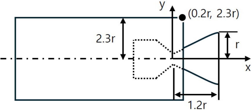
The CFD (Computational Fluid Dynamics) models employed in this study were based on a 10-ton-class rocket engine currently under development at KARI as an upper stage engine for next-generation launch vehicles. The simulations considered a scenario where a launch vehicle equipped with a single engine falls vertically. The 10-ton engine development model underwent ground combustion testing and was verified via CFD analysis for the design of a ground high-altitude simulation facility [37,38]. Due to the axisymmetric geometry of the launch vehicle and engine, a 2-D axisymmetric calculation was performed for computational efficiency. The simulations utilized Simcenter Star-CCM+ (version 2206), a commercial software based on a density-based coupled solver. For the CFD analysis, the engine model was configured with the same combustion chamber conditions but with a reduced nozzle expansion ratio of 16, as shown in Fig. 1. The nozzle length from the throat to the exit was set to 1.2r, where r represents the nozzle exit radius, and the launch vehicle body radius was 2.3r. The nozzle throat was centered on the central axis, and the body extended 0.2r rearward from the central axis.

Turbulence characteristics significantly influence CFD simulations of rocket engine flow and SRP. While LES (Large Eddy Simulation) provides detailed turbulent structures, RANS (Reynolds-Averaged Navier-Stokes) models are effective in predicting time-averaged flow features, making them suitable for SRP flowfield analysis [26]. Commonly used turbulence models in RANS solvers include the SA (Spalart-Allmaras) one-equation eddy viscosity model [26], Menter’s SST (Shear Stress Transport) k-ω model [20], and the standard k-ε two-equation model [39], depending on the characteristics of the solver. Among these, the realizable two-layer k-ε turbulence model, implemented in Star-CCM+, has demonstrated good agreement with hot-fire test results of rocket engines [37], and thus was adopted in this study. The retro-propulsive flow during descent involves supersonic exhaust interacting with the freestream, generating complex shock waves and boundary layer separations. To accurately capture both convective and diffusive flow phenomena, the AUSM (Advection Upstream Splitting Method) + FVS (Flux-Vector Splitting) scheme was used, providing second-order accuracy in the flow vector splitting. The AUSM + FVS scheme was well-suited for analyzing strong shocks and supersonic or hypersonic rarefaction waves [40].

Simulations were performed under implicit unsteady conditions. For steady-state analyses such as SPM, a time step of 10^-4 s was used, while for unsteady cases like LPM, a finer time step of 10^-6 s was applied. Temporal discretization was handled using a second-order scheme. Further details can be found in previous studies [37,38].

Fig. 1.

Launch vehicle model for numerical simulation.

2.2 Physical properties and computational grid conditions

The combustion chamber of the rocket engine operated at a stagnation pressure of 10 MPa and a stagnation temperature of 3,728 K. The thermophysical properties of the exhaust gases, which are products of combustion passing through the nozzle, were determined using the NASA CEA (Chemical Equilibrium with Applications) program. The resulting input properties for the CFD analysis were a molecular weight of 23.8 kg/kmol and a specific heat capacity of 1.88 kJ/(kg･K). For boundary conditions, sea-level atmospheric conditions were used for grid independence studies, while the SRP simulations assumed standard atmospheric conditions at 10 km altitude. Both air and exhaust gases were modeled as thermally perfect, non-reacting ideal gas mixtures. The temperature distribution in the reacting flow case was approximately 10% higher than that in the frozen case owing to additional heat release from post-combustion. Nevertheless, its impact on the overall flow field pattern was considered insignificant [41]. Accordingly, the present study focuses primarily on the flowfield characteristics and adopts the non-reacting mixing assumption.

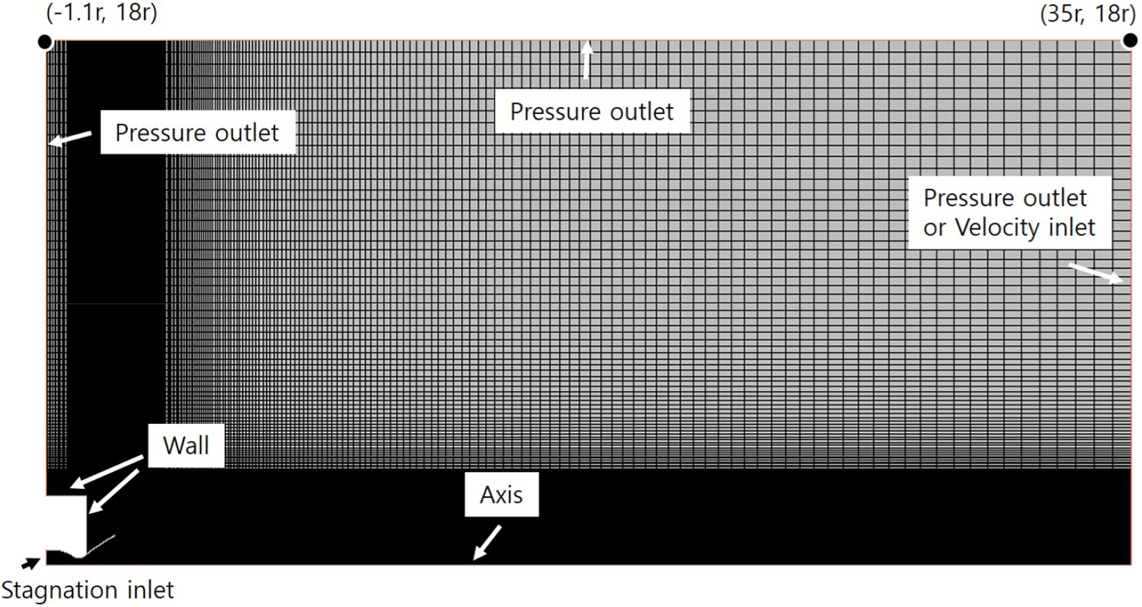
The validity of 2-D axisymmetric analysis for rocket engines has been verified in reference [37]. Furthermore, Reference 41 adopted a 2-D axisymmetric approach for the analysis of supersonic retro-propulsion of a launch vehicle under zero angle-of-attack conditions. Accordingly, the supersonic retro-propulsion flow induced by a single engine was assumed to be axisymmetric in the present study. In the 2-D axisymmetric simulation, the computational domain was defined as extending 18r in the y-direction and from -1.1r to 35r in the x-direction, with the nozzle throat as the center point, as illustrated in Fig. 2. Boundary conditions were set as follows: a stagnation inlet at the engine inlet, a pressure outlet for the ambient atmosphere, and wall boundaries for the nozzle and vehicle body. For descent simulations, the boundary downstream of the nozzle, aligned with the direction of vehicle motion, was set as a velocity inlet instead of a pressure outlet. A structured grid was employed, with the first cell height near walls set to 1 mm and y⁺ maintained below unity.

Fig. 2.

CFD grid and boundary conditions.

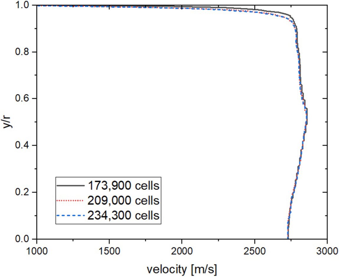
Under sea-level conditions, three different grid resolutions (173,900, 209,000, and 234,300 cells) were tested by comparing the nozzle exit velocity in Fig. 3. Within the core region (y/r = 0-0.8), velocity differences across grids were negligible. However, near the nozzle wall, minor variations were observed. The medium (209,000 cells) and fine (234,300 cells) grids produced nearly identical velocity distributions, while the coarse grid (173,900 cells) showed slight discrepancies. Therefore, the medium-resolution grid (209,000 cells) was adopted for all simulations.

Fig. 3.

Velocity distribution at the nozzle exit for grid resolution.

3. Results and Discussion

3.1 Nozzle Exhaust Flow Characteristics as a Function of Altitude

The exhaust flow characteristics of a rocket engine were investigated under external conditions corresponding to sea level and an altitude of 10 km. At the nozzle exit, the Mach number is approximately 3.53 and the temperature is about 1,600 K. The Mach number distributions for the two altitude conditions are presented in Fig. 4. At sea level, the exhaust jet expands immediately downstream of the nozzle exit and subsequently contracts. The first contraction point occurs at approximately 5r downstream, with a maximum radial expansion of about 1.5r from the centerline. In contrast, at 10 km altitude, the first contraction appears farther downstream at 12r, and the maximum expansion width increases to about 2.6r. Overall, the exhaust jet at 10 km expands nearly twice as much and extends more than twice as far as that at sea level. The internal Mach number also increases with altitude, producing a higher Mach distribution than under sea-level conditions. The centerline Mach number distributions are shown in Fig. 5. At sea level, the Mach number rises slightly from 3.53 at the nozzle exit to 3.7 at x/r = 2.5, then decreases to 2 at x/r = 5. Thereafter, the flow exhibits alternating acceleration and deceleration with gradually diminishing amplitudes. At 10 km altitude, the Mach number increases from 3.53 at the nozzle exit to 5.2 at x/r = 7.5, followed by a sharp drop to 2 at x/r = 10. Beyond this point, the flow continues to oscillate between acceleration and deceleration, with decreasing intensity. Due to under-expansion at higher altitude, the cycle length of acceleration and deceleration is approximately half of that observed at sea level.

Fig. 4.

Altitude-dependent Mach number contour inside the nozzle exhaust plume.

Fig. 5.

Mach number profiles on the nozzle exhaust gas centerline as a function of altitude.

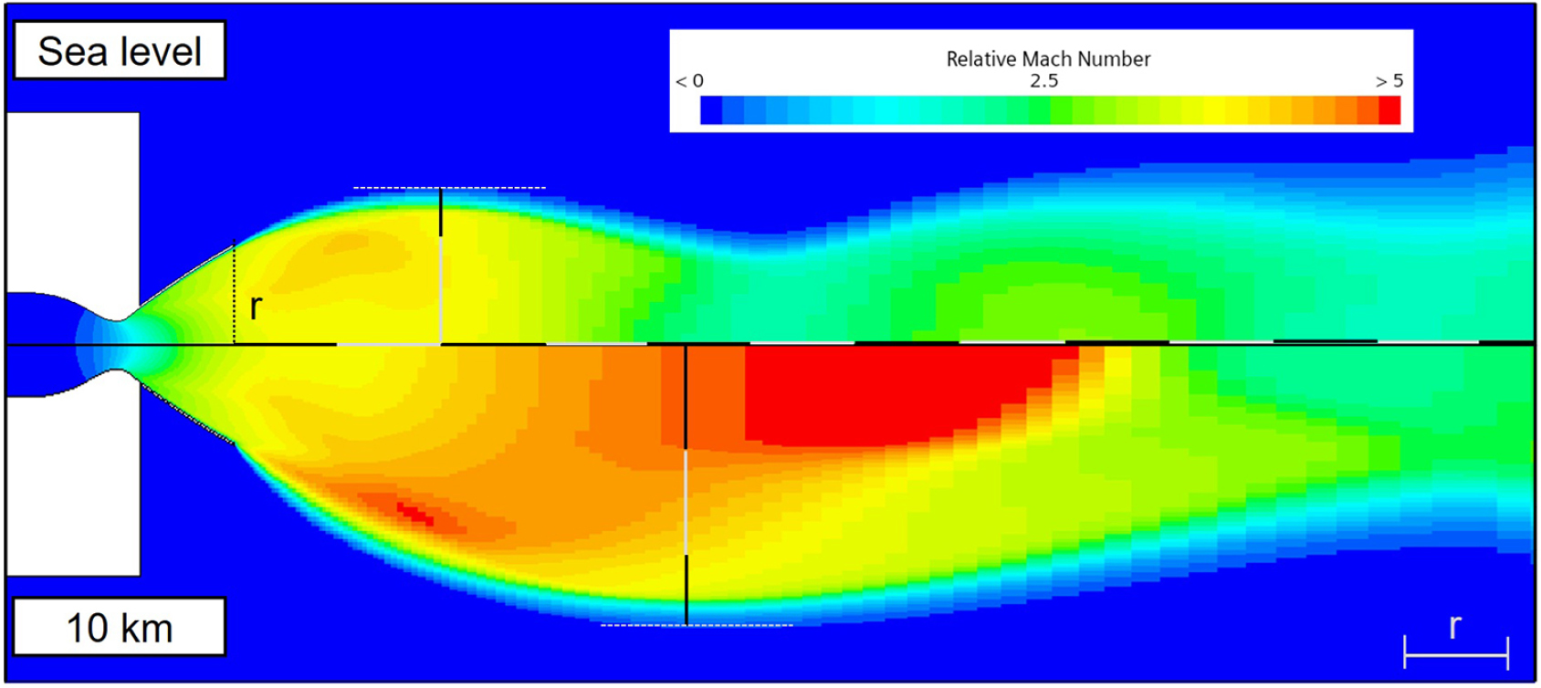
Fig. 6 presents the exhaust temperature distributions at the two altitudes. The centerline temperature at the nozzle exit is approximately 1,600 K. Owing to the under-expanded nature of the flow at 10 km, the wake region behind the nozzle exit exhibits lower temperatures compared with the sea-level case. At sea level, a localized high-temperature region (yellow) is observed near x/r = 6, whereas at 10 km altitude the exhaust temperature decreases significantly, reaching values close to 1,000 K (blue). At x/r = 12, the temperature distributions for both conditions become comparable. Fig. 7 illustrates the centerline temperature evolution. Under sea-level conditions, the temperature decreases from 1,600 K at the nozzle exit to 1,360 K at x/r = 2, then rises sharply to 2,500 K at x/r = 6. Beyond this point, the flow maintains temperatures above 2,000 K, displaying a distinct wavy pattern. At 10 km altitude, by contrast, the under-expanded jet causes the centerline temperature to fall from 1,600 K at the nozzle exit to 1,000 K at x/r = 8, before rising to 2,500 K at x/r = 12 and subsequently decreasing again. A comparison of Figs. 3 and 5 indicates an inverse correlation between the Mach number and temperature within the exhaust flow, with the magnitude of variation governed by the amplitude of the oscillations.

Fig. 6.

Altitude-dependent temperature contour inside the nozzle exhaust plume.

Fig. 7.

Temperature profiles on the nozzle exhaust gas centerline as a function of altitude.

3.2 Flow Characteristics in the Wake of the Rocket Body during Free Fall

In the absence of SRP jet flow from the rocket engine nozzle, the flow field around the wake of a free-falling launch vehicle was examined with respect to the flight Mach number. Fig. 8 presents the flow structures corresponding to flight Mach numbers ranging from 3.0 to 1.5, which are lower than the nozzle exit Mach number of 3.53. As the flight Mach number decreases, the bow shock moves downstream from the nozzle exit, and its inclination angle increases. Within the nozzle, as well as in the region between the nozzle lip and the rocket base, the Mach number contours remain dark blue, indicating nearly stagnant flow. Along the nozzle lip and trailing edge of the rocket base, a light blue Mach number contour appears. At M_flight = 3.0 and 2.0, the flow past the nozzle lip impinges on the rocket base shoulder, producing a light green Mach number contour along the base wall. At M_flight = 1.7, however, the flow undergoes a rapid expansion at the base shoulder, leading to locally elevated flight Mach numbers. In this condition, flow separation occurs near the base shoulder, resulting in dark-blue contours close to the wall, indicative of very low velocities. The bow shock location as a function of flight Mach number is summarized in Fig. 9, showing a nearly linear trend. At M_flight = 3.0, the bow shock is located at x/r = 0.9, whereas at M_flight = 1.5 it is displaced downstream to x/r = 2.3, confirming that the bow shock moves farther from the nozzle exit as the flight Mach number decreases.

Fig. 8.

Mach number contour on the aft section of the launch vehicle as a function of descending flight Mach number.

Fig. 9.

Variation of bow shock location with descending flight Mach number.

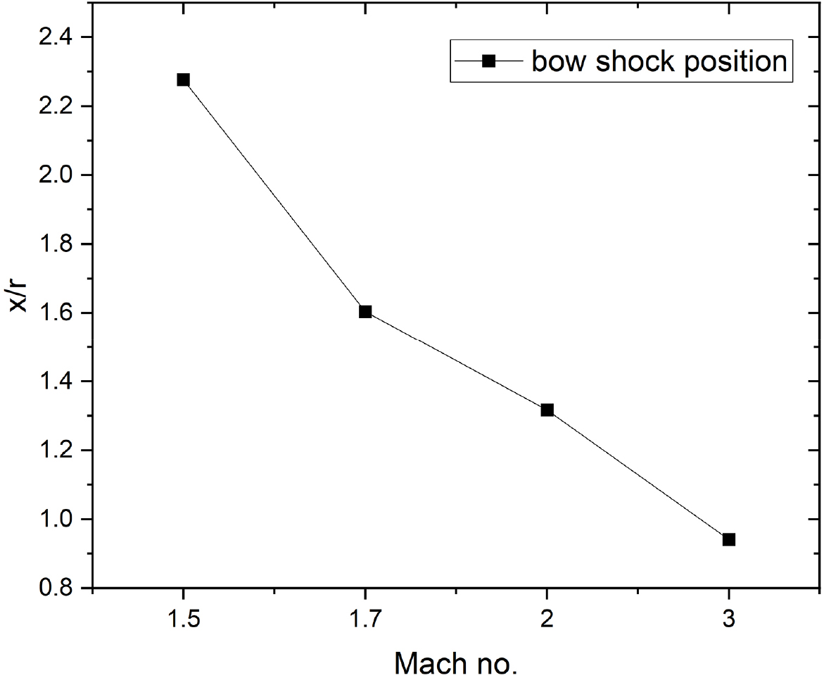
Fig. 10 illustrates the distribution of turbulent viscosity around the rocket base. Turbulent viscosity is not a physical property but rather a modeled quantity representing the momentum transport effect of turbulent eddies, typically approximated as a viscous term. In the standard k-ε turbulence model, it is expressed as in Eq. (1)[39], where the turbulent viscosity (μ_t) is a function of the turbulent kinetic energy (k), density, turbulent dissipation rate (ε), and an empirical constant (C_μ).

Fig. 10.

Turbulent viscosity contour around the aft body of the launch vehicle as a function of descending flight Mach number.

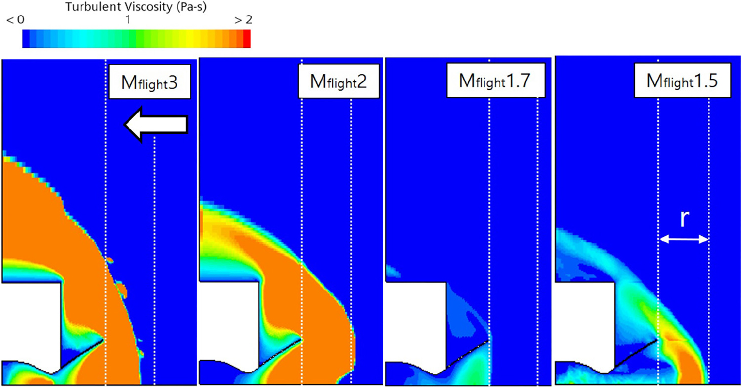
At M_flight = 3.0, turbulent viscosity is strongly developed along the bow shock and extends into the nozzle interior. Notably, high levels of turbulent viscosity also appear near the nozzle throat within the combustion chamber, induced by the flow ingested from the nozzle. Along the bow shock structure, most of the rocket base region is characterized by high turbulent viscosity. At M_flight = 2.0, a recessed region of strong turbulent viscosity develops from the bow shock center toward the nozzle interior. Although turbulent viscosity remains intense along the bow shock structure, its magnitude weakens toward the rocket forebody compared with the point of shock initiation. At M_flight = 1.7, the flow characteristics deviate markedly from those at flight Mach numbers 2.0 and 3.0. Turbulent viscosity is concentrated mainly at the nozzle exit and within the nozzle interior, and its magnitude is considerably reduced. At M_flight = 1.5, turbulent viscosity reappears strongly, but originates near r downstream of the nozzle exit. From Fig. 8, the bow shock at M_flight = 1.5 initiates at approximately 1.6r, suggesting that the turbulent viscosity distribution is influenced by nozzle-shock interactions. Flow passing through the bow shock interacts with the nozzle structure, generating bright-blue regions of turbulent viscosity inside the nozzle and even within the combustion chamber. The turbulent viscosity formed near 1r downstream of the nozzle exit propagates into the base region, gradually decaying in strength.

The wall-temperature distributions at the rocket base are shown in Fig. 11 for various flight Mach numbers. At M_flight = 3.0, the mean temperature on the rocket base wall is approximately 620 K. At M_flight = 2.0, the base wall maintains a nearly uniform temperature of 400 K. At M_flight = 1.7, the temperature is slightly above 400 K and remains steady until y/r = 1.0, after which it decreases to about 350 K. At M_flight = 1.5, the wall temperature starts at 450 K, rapidly decreases to about 340 K by y/r = 0.75, and then gradually decreases further.

Fig. 11.

Effect of descending flight Mach number on the temperature distribution on the aft face of the launch vehicle.

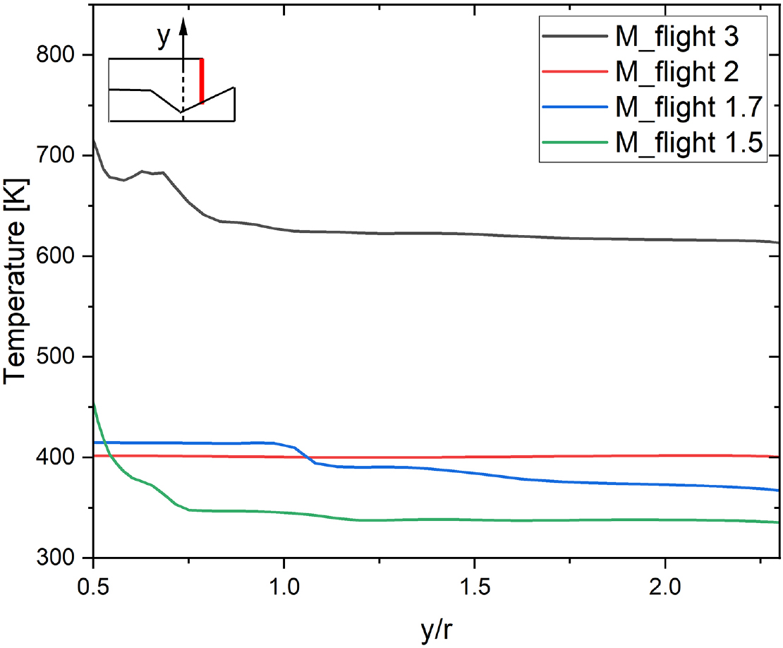
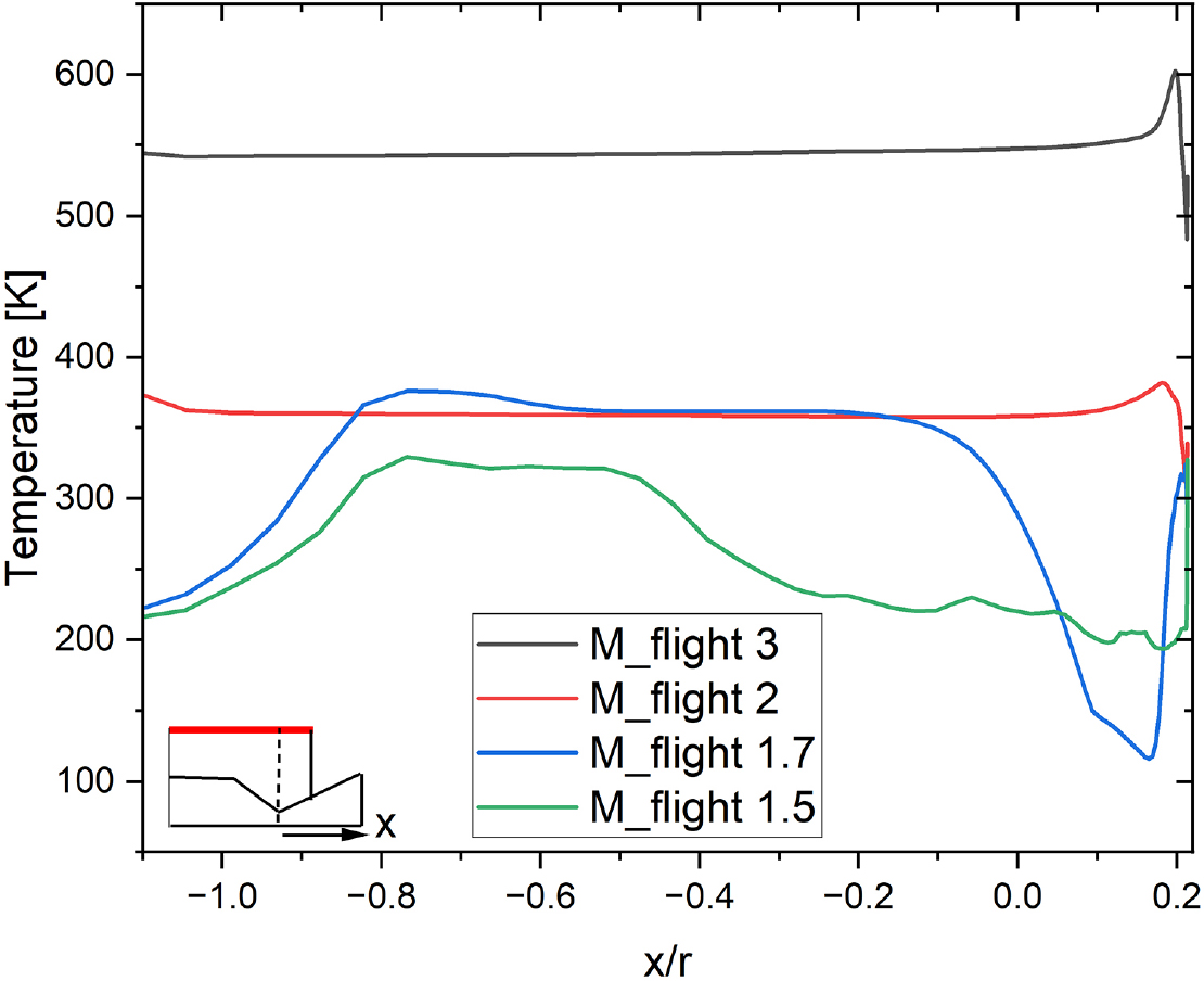
Fig. 12 presents the temperature distribution along the rocket base sidewall. At M_flight = 3.0, the sidewall exhibits a uniform temperature of approximately 550 K. At M_flight = 2.0, the temperature is uniformly distributed at about 350 K. At M_flight = 1.7, the sidewall temperature increases from 220 K to about 350 K near x/r = -0.8, remains constant until x/r = -0.1, then abruptly decreases to about 100 K before rising again to 300 K. This trend reflects the generation of a strong expansion wave at the base shoulder, as observed in Fig. 8, causing a rapid temperature drop in the adjacent wall region. At M_flight = 1.5, the temperature increases from 220 K to about 330 K near x/r = -0.8, then gradually decreases to about 200 K beyond x/r = -0.5. Although weaker, this trend is similar to that observed at M_flight = 1.7, where expansion-induced cooling occurs because the separated flow prevents the base wall from being significantly affected by the bow-shock-heated flow.

Fig. 12.

Effect of descending flight Mach number on the temperature distribution on the side face of the launch vehicle.

3.3 Flow Characteristics around the Rocket Afterbody Induced by SRP during Descent Flight

During descent flight with SRP, various parameters, such as the operating conditions of the SRP engine and variations in the flight Mach number, must be considered. As noted in the introduction, the thrust coefficient [20] and the MFR (Momentum Flux Ratio) [18] are commonly employed to characterize these effects. This study employs MFR and flight Mach number as the variables. The definition of MFR is provided in Eq. (2)

Here, u is the velocity, and ρ is the density. The subscript a denotes ambient conditions, and e represents the nozzle exit.

To investigate the influence of SRP during vehicle descent, the flight Mach number was varied from 4.0, which is higher than the exhaust Mach number at the nozzle exit, down to 1.4, within the lower supersonic regime. With fixed engine conditions, MFR increases as the flight Mach number decreases.

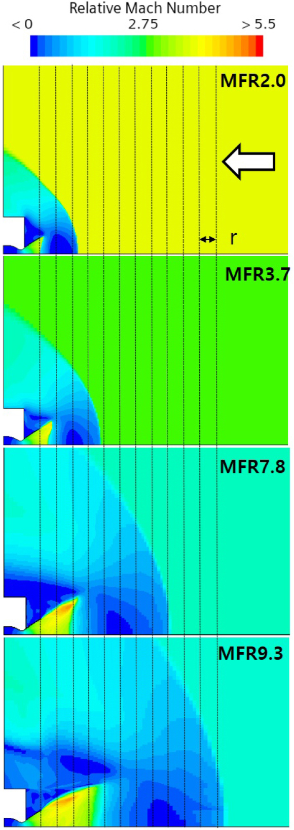
Fig. 13 compares the Mach number contours as functions of either MFR or the freestream Mach number. Overall, as MFR increases, the bow shock moves farther downstream from the nozzle exit, and the exhaust plume penetrates further aft. At MFR = 2.0, the bow shock is located at 2r from the nozzle exit. Due to the high freestream Mach number, the exhaust plume remains close to the nozzle exit, while the after-body side flow is mostly supersonic. At MFR = 3.7, the bow shock is located at 4r from the nozzle exit; the plume penetrates farther downstream, although the plume front exhibits a concave vertical shape. At MFR = 7.8, the bow shock forms at 8r, with a larger shock angle, and a subsonic region (dark blue) develops near the vehicle sidewall. The plume expands radially up to 2r from the nozzle exit. The increased penetration of the plume accelerates the outer shear layer, yielding higher Mach number regions (orange). At MFR = 9.3, the bow shock forms at 11r, and the plume penetration length increases to 4r. However, compared with MFR = 7.8, the sidewall flow exhibits a more unstable distribution.

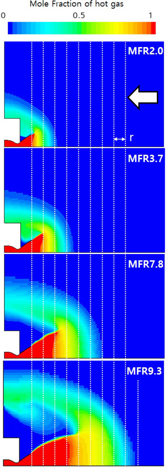
The mole fraction distributions of the exhaust gases are presented in Fig. 14. At MFR = 2.0, the exhaust plume extends to 2r, coinciding with the bow shock location, and the distribution is similar in shape to the shock profile. The plume concentration is highest near the nozzle exit and decreases toward the after-body. At MFR = 3.7, the plume penetrates to 4r, again showing similar behavior to the bow shock. In both cases (MFR = 2.0 and 3.7), the exhaust plume fills the recirculation region behind the after-body and remains in contact with the vehicle sidewall. At MFR = 7.8, the plume extends to 6r, but it does not re-enter the aft recirculation region and instead separates from the sidewall. The bow shock, located at 8r (Fig. 13), lies farther downstream than the exhaust penetration, and thus the plume does not reach the bow shock. From MFR = 7.8 onward, the bow shock location and the exhaust concentration distribution no longer coincide. At MFR = 9.3, the plume extends to 9r, showing an under-expanded flow structure directed downstream. Flow separation occurs near the after-body corner, producing vortical structures. The bow shock forms at 11r (Fig. 13), and, as with MFR = 7.8, the exhaust gases do not penetrate up to the bow shock.

Fig. 13.

Mach number contour around the after-body for different MFR values.

Fig. 14.

Mole fraction contour around the after-body for different MFR values.

The temperature distributions around the after-body for varying MFR are shown in Fig. 15. The exhaust plume undergoes deceleration and temperature rise across the Mach disk. Consequently, downstream of the Mach disk, the flow transitions from supersonic to subsonic (dark blue in Fig. 13) and exhibits high-temperature regions (yellow). As MFR increases, the high-temperature region induced by the Mach disk extends further downstream. At MFR = 2.0, the high-temperature region reaches 2r, coinciding with the bow shock and exhaust distribution in Fig. 13. At MFR = 3.7, it extends to 4r, showing a similar trend. In these cases, the Mach number distribution across the bow shock and the temperature field exhibit consistent behavior, and the hot exhaust gases directly affect the after-body base and sidewall regions. At MFR = 7.8, the high-temperature region extends to 7r. The plume distribution (Fig. 14) reaches 6r, while the bow shock (Fig. 13) is located at 8r; thus, the temperature field extends between these two regions. Since the plume does not reach the bow shock, the high-temperature region remains separated from the after-body, although the recirculation behind the nozzle maintains a hot-gas environment near the base. At MFR = 9.3, the high-temperature region extends to 10r, between the plume penetration (9r in Fig. 14) and the bow shock location (11r in Fig. 13). The hot plume induces heating nearly up to the bow shock. However, similar to MFR = 7.8, the plume does not significantly affect the after-body base, as the flow is separated and vortical.

The turbulent viscosity distributions with increasing MFR are shown in Fig. 16. At MFR = 2.0, turbulent viscosity is strongly concentrated near 2r and follows the bow shock structure, owing to the interaction between the Mach disk and bow shock. At MFR = 3.7, the turbulent viscosity extends to 4r but is weaker than at MFR = 2.0, still following the bow shock. At MFR = 7.8, the turbulent viscosity extends up to 7r. Although the distribution broadens, the intensity diminishes as the bow shock weakens; thus, no turbulent viscosity is observed along the sidewall or after-body base. Comparison with Fig. 14 (plume distribution to 6r) and Fig. 13 (bow shock at 8r) indicates that turbulent viscosity is primarily governed by the interaction between the plume and the Mach disk. At MFR = 9.3, turbulent viscosity extends to 8r and appears stronger farther downstream from the nozzle exit. This again demonstrates its dependence on the Mach disk. No significant turbulent viscosity is observed near the after-body wall or base. A comparison of Figs. 15 and 16 indicates that high-temperature regions correspond to zones where the plume is decelerated by the Mach disk, while turbulent viscosity increases in response to unsteady flow features induced by the Mach disk.

Fig. 15.

Temperature contour around the after-body for different MFR values

Fig. 16.

Turbulent viscosity contour around the after-body for different MFR values.

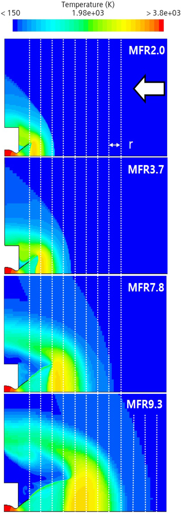
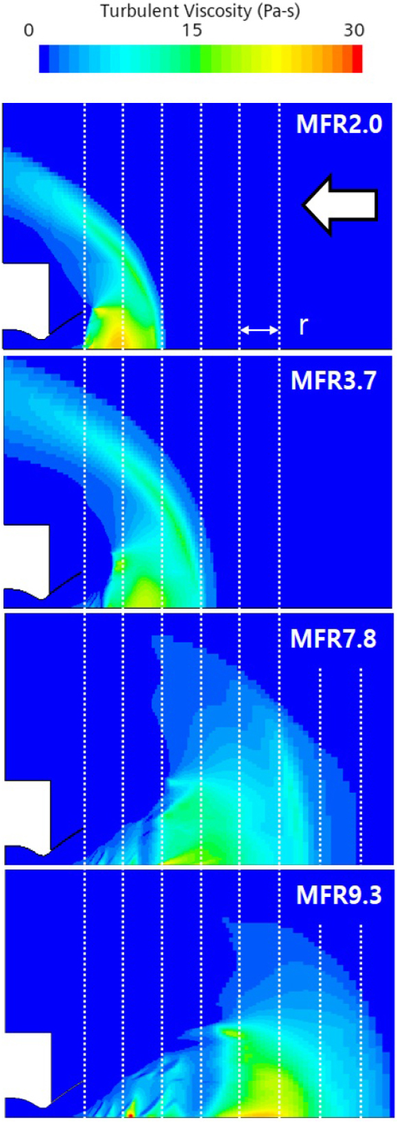
Fig. 17 illustrates the temperature distribution along the vehicle sidewall as a function of MFR. For MFR = 2.0 and 3.7, a high temperature of approximately 2,250 K is maintained uniformly. This is because, as shown in the temperature contours in Fig. 15, the hot exhaust gases from the nozzle cover both the base and the sidewall of the after-body. In contrast, for MFR = 7.8 and 9.3, the sidewall maintains a uniform temperature of about 250 K, since the hot exhaust plume flows separated from the after-body, as indicated in Fig. 15.

Fig. 17.

Temperature distribution along the side wall of the after-body for different MFR values.

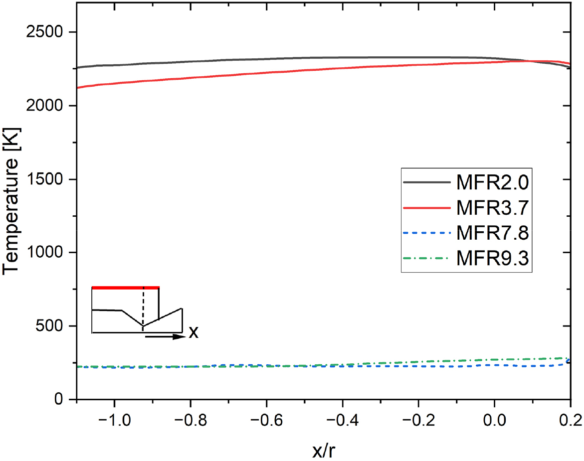
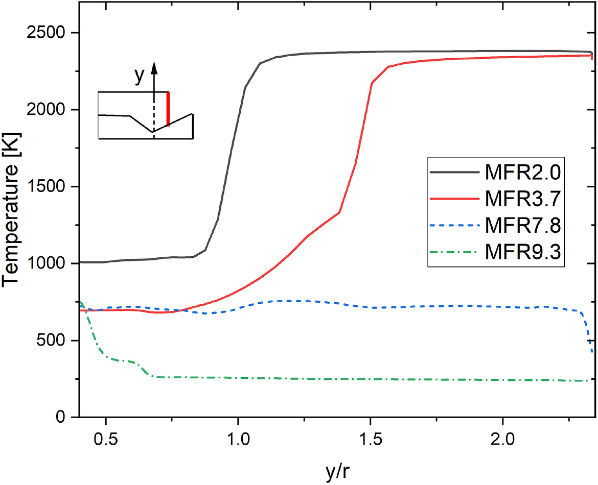
Fig. 18 presents the temperature distribution at the after-body base. At MFR = 2.0, the base temperature begins at approximately 1,000 K and rises sharply from y/r = 0.8, reaching about 2,250 K near y/r = 1.1, where it then stabilizes. At MFR = 3.7, the temperature starts at about 750 K and increases gradually, before sharply rising at y/r = 1.4 to reach a nearly constant value of approximately 2,250 K. In both cases, consistent with the observations in Fig. 15, the high-temperature nozzle exhaust directly impinges on the base region, resulting in significant thermal loading on the after-body. At MFR = 7.8, the base temperature remains constant at approximately 750 K. Although the main exhaust plume separates from the after-body (Fig. 15), the recirculating flow in the base region accounts for this temperature distribution. At MFR = 9.3, the base temperature decreases from about 750 K to 250 K. As shown in Fig. 15, the deflection point of the nozzle exhaust due to the bow shock shifts farther away from the after-body base, and the influence of hot-gas recirculation is minimal. Consequently, the base region exhibits this lower temperature distribution.

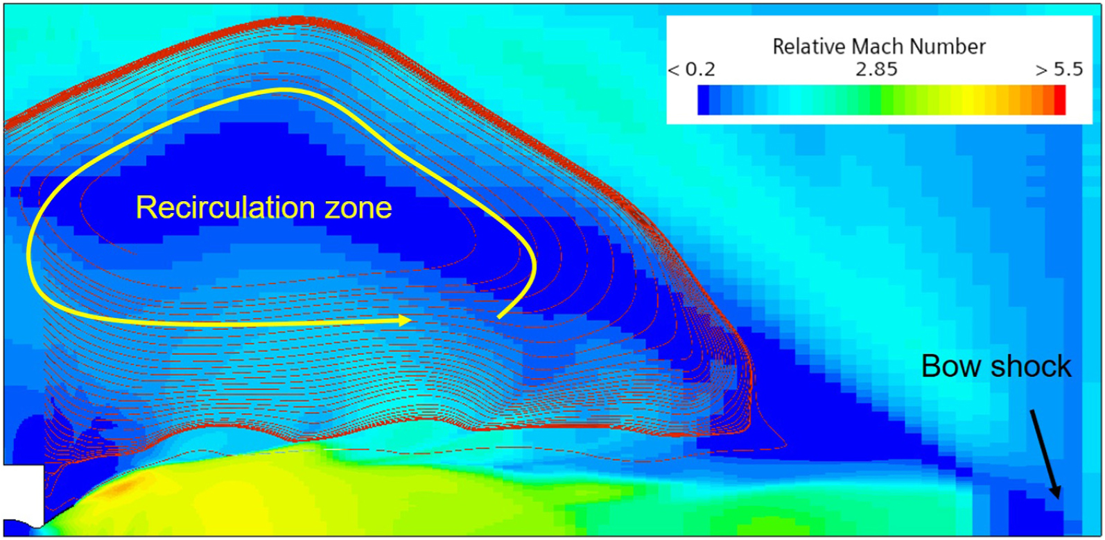
At MFR 11.2, it is observed that the flow pattern, which had previously exhibited SPM, transitions into LPM, as illustrated in Fig. 19. The LPM is not steady but inherently unsteady, and the Mach number distribution presented corresponds to an instantaneous snapshot at a specific time. The nozzle exhaust plume is considerably elongated, and a weak bow shock is formed at its downstream end. Owing to the influence of this bow shock, an inclined shock structure emerges near the centerline. Furthermore, flow separation is identified in the outer region of the exhaust jet, within the inclined bow shock region. A large-scale recirculation zone develops between the inclined bow shock structure and the exhaust jet, leading to unstable flow characteristics in the vicinity of the exhaust plume.

Fig. 18.

Temperature distribution along the rear wall of the after-body for different MFR values.

Fig. 19.

Mach number contour at MFR 11.2 in LPM.

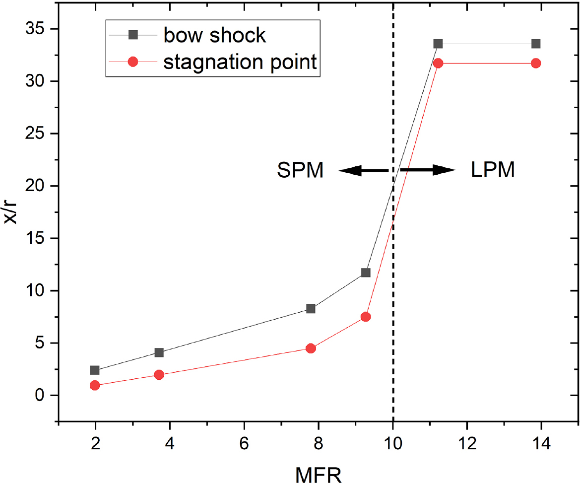
The transition between SPM and LPM with respect to MFR is compared in Fig. 20. For the present rocket engine model, it is found that, as MFR increases, both the bow shock and the stagnation point increase proportionally. Beyond approximately MFR 10, however, the variations in the bow shock and stagnation point become insignificant, and the flow transitions into LPM. The cases of MFR 9.8 (M_flight = 1.8) and MFR 11.2 (M_flight = 1.7) indicate that the transition point is highly sensitive when interpreted in terms of Mach number. In SPM, the transitional regime between MFR 3.7 (M_flight = 3) and MFR 7.8 (M_flight = 2) exhibits noticeable differences in the nozzle-exit flow properties, including Mach number, temperature distribution, and turbulent viscosity. At MFR < 3.7, direct interference between the bow shock and the exhaust plume occurs near the nozzle exit, exerting a dominant influence on the surrounding flow structures. At MFR 7.8, the effect of the bow shock is considerably weakened, whereas the influence of the exhaust plume—particularly that associated with the Mach disk—becomes dominant. With a further increase in MFR, the contribution of the bow shock continues to diminish, while the impact of the exhaust plume becomes increasingly significant, ultimately resulting in the transition from SPM to LPM. In other words, as the flight Mach number decreases from a high supersonic regime to the transonic regime, the momentum of the incoming flow that obstructs the supersonic nozzle exhaust decreases, thereby altering the flow interaction.

Fig. 20.

Mode transition as a function with MFR.

4. Conclusion

A small launch vehicle equipped with a rocket engine operating at a chamber pressure of 10 MPa and a nozzle exit Mach number of 3.53 was considered in free fall. The flow characteristics around the base body and nozzle under SRP were analyzed using CFD simulations as a function of the descending flight Mach number. Based on the CFD results, the flow behavior corresponding to various free-fall Mach numbers, assuming a fixed nozzle exit Mach number, can be summarized as follows:

(1) In the case of vertical free fall without SRP, the bow shock moves downstream from the nozzle exit and its strength decreases as the flight Mach number decreases. At higher Mach numbers, turbulent viscosity is enhanced due to the bow shock, which in turn affects the nozzle interior as well as the base body. When the Mach number is high, the bow shock remains close to the nozzle exit, and aerodynamic heating leads to elevated wall temperatures along the side and rear surfaces of the base body.

(2) Under SRP, the flow characteristics around the base body and nozzle were investigated as a function of the flight Mach number and the exhaust flow condition parameter MFR. For MFR values between 2.0 and 3.7, direct interaction occurs between the bow shock and the nozzle exhaust plume. Consequently, the high-temperature exhaust gas envelops the side and rear surfaces of the base body, exposing the wall to temperatures exceeding 2,000 K.

(3) As MFR increases from 7.8 to 9.3, the interaction around the base body is governed primarily by the exhaust plume rather than by the free-stream Mach number. In this regime, the spatial distribution of the exhaust plume does not coincide with the position of the barrel shock. The Mach disk formed within the exhaust plume induces increased turbulent viscosity and temperature rise in the plume’s wake. On the side surface of the base body, relatively low wall temperatures are observed since the exhaust plume wake detaches from the body. Although the recirculating flow behind the base body still interacts with the hot exhaust gases, the wall temperature at the rear surface is lower than in the low-MFR cases.

(4) When MFR exceeds 10, the flow field resulting from the interaction between the retro-jet and the free-stream transitions from SPM to LPM. In this case, the nozzle exhaust jet becomes highly elongated, and a weak bow shock forms at its downstream end. Large-scale recirculation zones develop between the inclined shocks generated by the bow shock and the exhaust jet, leading to flow separation and unstable recirculating structures around the nozzle plume. As descending flight Mach number decreases from a high supersonic regime to the transonic regime, the momentum of the incoming flow that obstructs the supersonic nozzle exhaust decreases, thereby altering the flow interaction.

(5) In general, for MFR ≤ 5, the nozzle exhaust directly interacts with the bow shock, and the resulting flow structures significantly influence the entire base body. For MFR > 5, the flow field is predominantly governed by the nozzle exhaust plume, and flow structures such as shocks are formed further downstream of the nozzle exit. In this regime, the influence of the high-temperature exhaust plume on the base body is reduced. For MFR > 10, the exhaust plume extends farther downstream and transitions into LPM, exhibiting flow structures characteristic of those observed during landing burns.